Introduction
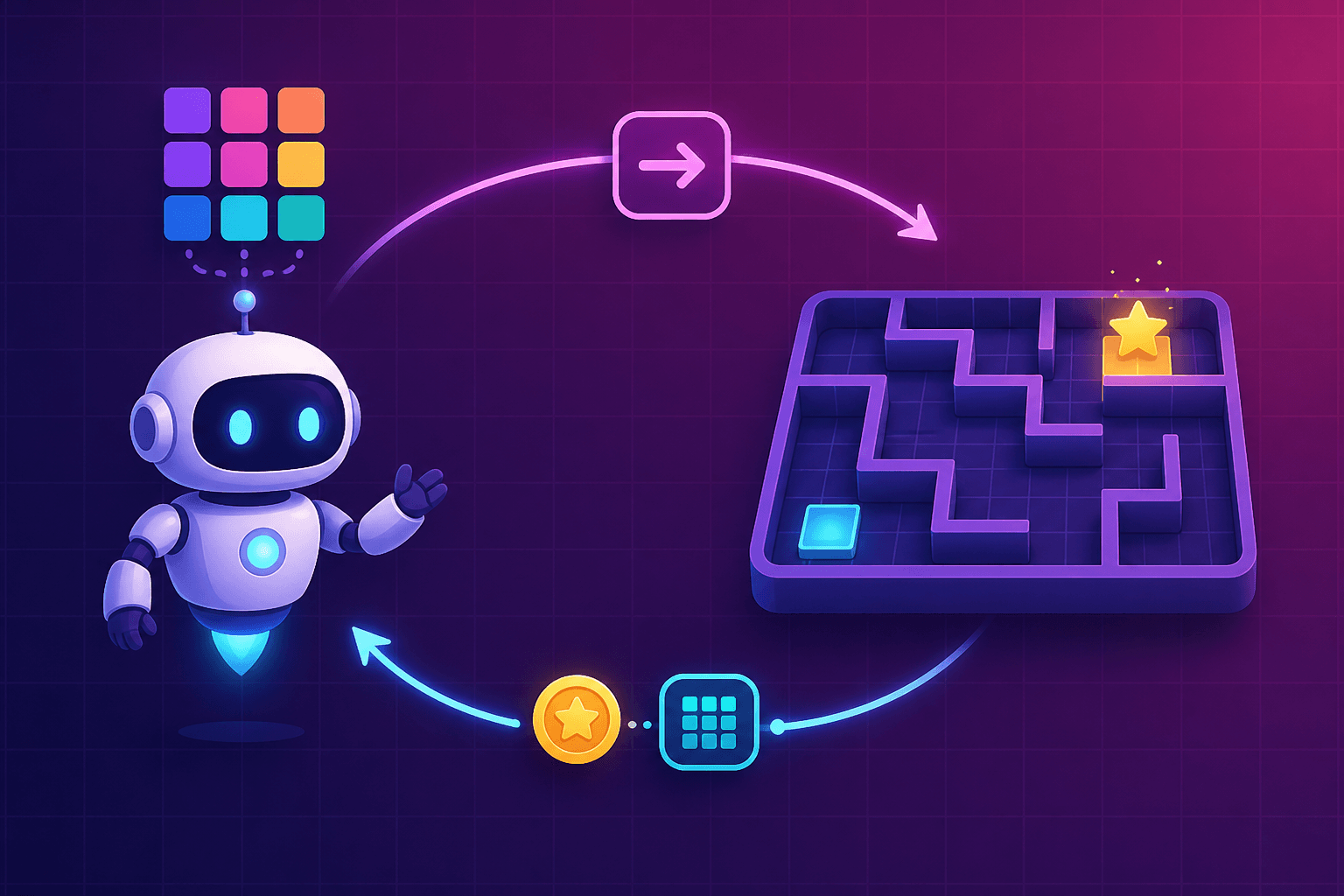
Reinforcement learning studies agents that learn from interaction: given a state, pick an action, receive a reward, repeat. The framework — a Markov Decision Process — is deceptively small and hides real subtlety around exploration, credit assignment, and off-policy correction.
Modern successes (AlphaGo, RLHF for language models, robotics) all rely on the ideas below. Interview questions typically test whether you understand the *tradeoffs*: on-policy vs off-policy, model-based vs model-free, value vs policy, greedy vs stochastic.
01
Fundamentals & MDPs
56 conceptsDefine the RL setting: agent, environment, state, action, reward, policy.
easy- An agent observes a state s from the environment, picks an action a via its policy , receives a reward r and a new state s'.
- The goal is to maximize the expected cumulative discounted reward (return).
- Formalized as a Markov Decision Process (S, A, P, R, gamma).
- The agent learns pi (or a value function) from interaction with the environment.
On-policy vs off-policy learning — what's the difference?
medium- On-policy methods learn from data generated by the current policy (e.g., SARSA, REINFORCE, PPO).
- Off-policy methods learn from data collected by a different (behavior) policy — this enables replay buffers and reusing old data (e.g., Q-learning, DQN, SAC, DDPG).
- Off-policy is more sample-efficient; on-policy is often more stable and easier to tune.
What does the Bellman equation say?
medium- For a policy pi: .
- For the optimal value: E[r + gamma · V*(s')].
- It expresses the value of a state as the immediate reward plus the discounted value of the next state.
- Solving the Bellman equation is the core of dynamic programming, TD learning, and Q-learning.
What role does the discount factor gamma play?
easy- Gamma in [0, 1) weights how much future rewards matter compared to immediate ones.
- Gamma close to 0 = myopic (only care about immediate reward); gamma close to 1 = far-sighted (care about long-term).
- Also ensures the return sum converges in infinite-horizon problems.
- Choose based on the task horizon and stability of value estimates.
What is the credit assignment problem?
hard- In sequential tasks with delayed rewards, it's hard to know which past action caused a given reward.
- Long horizons, sparse rewards, and stochasticity make it worse.
- Methods that help: temporal-difference learning, eligibility traces, n-step returns, GAE (generalized advantage estimation), and hindsight experience replay.
Model-based vs model-free RL — when do you prefer each?
medium- Model-based RL learns a model of the environment (transitions and rewards) and uses it to plan (e.g., MuZero, Dreamer).
- It is more sample-efficient — great when real interactions are expensive (robotics, healthcare).
- Model-free RL learns policy or values directly from experience — simpler, and it wins when the environment is complex/hard to model.
- Modern successes often combine both.
What is the Markov property and why does it matter?
medium- — the future depends only on the current state, not the history.
- Enables efficient RL: policy and value functions depend on state alone, not history.
- When violated (partial observability), we use POMDPs, recurrent nets, or state-stacking (Atari frame stack) to recover a Markovian representation.
POMDP — how does it differ from MDP?
hard- Partially Observable MDP: agent observes which gives incomplete info about state .
- Add observation function .
- Belief state b(s) = posterior over s given history → sufficient statistic for optimal policy.
- Solving POMDPs is PSPACE-hard exactly; approximate via RNN/LSTM encoding of history, or particle filter beliefs, or transformer over recent observations.
- Realistic robotics / partial-info games.
V(s) vs Q(s, a) — the difference.
easy- V(s) = expected return from state s following policy π.
- Q(s, a) = expected return from state s taking action a THEN following π.
- Relationship: Q(s, a).
- Optimal: Q*(s, a).
- Q allows action selection without a model (Q-learning); V requires a model to compute argmax over actions.
- Actor-critic methods often estimate V (simpler) but use per-action advantage A = Q - V.
What is the advantage function?
medium- A(s, a) = Q(s, a) - V(s) → how much better is action a than the average action in state s.
- Reduces variance in policy-gradient estimates (baseline subtraction preserves the gradient in expectation but shrinks variance).
- Standard estimators: TD-residual A ≈ r + γ V(s') - V(s) (biased low variance); n-step or GAE for bias-variance tradeoff.
- Used in A2C, PPO, TRPO.
Different notions of return — MC, TD(0), n-step, GAE.
hard- MC return: — full episode, unbiased, high variance.
- TD(0): — biased (bootstrap), low variance. n-step: + ... + — knob n interpolates.
- GAE (Generalized Advantage Estimation): weighted sum over n-step advantages with parameter λ — smooth bias-variance tradeoff.
- GAE with λ ≈ 0.95 is default in PPO.
What is TD error?
medium- — difference between the bootstrapped target and current estimate.
- Drives all TD-based updates: V ← V + α δ, Q-learning target is δ with max in bootstrap.
- Positive δ = state was better than expected; negative = worse.
- Fundamental signal for value learning.
- Modern uses: PPO advantage, GAE, prioritized replay weighting (δ magnitude).
Policy iteration vs value iteration.
medium- Policy iteration: alternate (a) policy evaluation , (b) policy improvement .
- Converges in finite steps.
- Value iteration: V ← (r + γ V(s')) repeatedly — combines both in one step.
- Value iteration is a special case of policy iteration with only one evaluation sweep.
- Both are dynamic programming, require the model.
TD(λ) — how does it work?
hard- Interpolates between TD(0) (λ=0, low variance biased) and MC (λ=1, unbiased high variance).
- Uses eligibility traces that decay by γλ each step and increment at visited states.
- Update: V(s) ← V(s) + α δ e(s) for every s.
- Online, single-pass, works with function approximation.
- Foundation of Sutton-Barto RL; GAE is essentially TD(λ) for advantages.
Monte Carlo methods in RL — when to use?
medium- Estimate V_π(s) or Q_π(s, a) via sample-average returns from full episodes.
- Unbiased (no bootstrap error), but only usable in episodic tasks + high variance.
- Every-visit MC: average over every visit to s in an episode.
- First-visit MC: only first occurrence.
- Rare in modern deep RL (TD methods better for long / continuous tasks) but foundation of return-conditioned methods and offline RL (Decision Transformer).
Tabular vs function-approximation RL — the challenge.
hard- Tabular: one entry per (s, a) — convergence guaranteed but doesn't scale.
- Function approximation (neural nets): scales to huge state spaces but breaks convergence guarantees.
- The 'deadly triad': off-policy + function approximation + bootstrapping → potential divergence.
- Modern deep RL uses tricks (target networks, replay, gradient clipping) to work despite the triad.
- Understanding this trap is key.
Why do Bellman operators converge?
hard- Bellman operator T is a γ-contraction in the max norm: ||||_∞ ≤ γ ||||_∞.
- By Banach fixed-point theorem, iterating T converges to unique fixed point V* at rate .
- Underlies value iteration, TD(0) convergence in tabular case, policy iteration.
- Function approximation can break the contraction (projected Bellman operator may not contract) → divergence.
TD vs MC — how they differ in bias-variance.
medium- MC: use full episodic return → unbiased estimator of V_π, but high variance (many random rewards over full trajectory).
- TD(0): use V(s') → biased (bootstrap error from imperfect V estimate) but lower variance (only one reward). n-step and TD(λ) interpolate.
- Choice: TD when episodes are long or variance dominates, MC when bias is intolerable + episodes short.
Linear function approximation for value functions — pros and cons.
medium- V(s) ≈ w'φ(s) with hand-crafted features φ.
- Convergence guarantees under on-policy (LSPI, LSTD) but poor scaling; requires domain-designed features.
- Baird's counterexample: off-policy + linear FA + bootstrap → divergence.
- Foundation of classic RL theory (Sutton, Bertsekas), superseded by neural nets in practice.
- Still valuable in tiny state spaces, small-embedded systems, or theoretical proofs.
When does tabular Q-learning provably converge?
hard- (1) All (s, a) visited infinitely often (adequate exploration), (2) Learning rate α satisfies Robbins-Monro: Σα = ∞, < ∞, (3) Bounded rewards.
- Under these, → Q* almost surely.
- Real deep-RL breaks (1) severely (state space huge) and mostly ignores (2).
- Classical theory guides intuition but doesn't guarantee anything in modern deep RL — that's why empirical care matters.
When does tabular Q-learning fail in practice?
medium- (1) State space too large: even discretized MazeGrid > 1M states makes tabular infeasible.
- (2) Continuous features: discretization fights curse of dimensionality.
- (3) Function structure across states unexploited (Q for nearby states should be similar → NN generalizes; tabular treats them independently).
- (4) Slow: no generalization means each state must be visited separately.
- Every real RL problem > toy uses function approximation (usually NN).
Why is subtracting a baseline OK in policy gradient?
hard- Because for any function b(s) independent of a.
- This adds no bias but shrinks variance by centering the reward signal.
- Choice of baseline: constant, moving average of returns, or state-dependent V(s) (best — cancels state-level variance).
- Advantage function A(s, a) = Q(s, a) - V(s) is the popular choice → gives us actor-critic architectures.
The log-derivative trick — why is it central to policy gradients?
hard- For expectation of f under π_θ: ∇_θ E_π[f] = E_π.
- Enables Monte Carlo estimation of gradient using only samples from π and gradient of log-likelihood — no need to differentiate through the reward function or the environment.
- Foundation of REINFORCE, actor-critic, natural gradient, and importance sampling.
- Trick: π_θ(x) ∇_θ log π_θ(x) = ∇_θ π_θ(x).
What is natural gradient in policy gradient methods?
hard- Follow the direction of steepest ascent in policy space measured by KL divergence (Fisher information metric) instead of Euclidean.
- Update: θ ← θ + α ∇J where F is Fisher information matrix.
- Invariant to reparameterization.
- Foundation of TRPO (approximate) and NPG.
- Practically: expensive — use Conjugate Gradient (TRPO) or K-FAC.
- Underpins why PPO's clipping approximates a trust region.
Reparameterization trick in stochastic policies.
hard- For continuous stochastic policy π_θ, sample a = μ + σ ⊙ ε with ε ~ N(0, I) → gradient flows through μ, σ directly.
- Enables low-variance path-wise gradients rather than score-function REINFORCE-style gradients.
- Used in SAC.
- Also foundation of VAEs.
- Doesn't work directly for discrete actions (use Gumbel-softmax as continuous relaxation).
GAE — Generalized Advantage Estimation formula.
hard- ^∞ where . λ = 0 → TD(0) advantage (biased, low var). λ = 1 → MC advantage (unbiased, high var).
- Typical λ = 0.95 in PPO.
- Provides smooth bias-variance tradeoff.
- Compute efficiently backward from end of trajectory.
- Standard advantage estimator in modern policy gradient methods.
Off-policy policy gradient — how does importance sampling enter?
hard- Data collected under behavior , but want to update target π_θ: use importance weight ρ = π_θ → ∇J ≈ E_π_b[ρ ∇log π_θ · A].
- Weight variance explodes when π_θ far from .
- Solutions: clip ratio (PPO), truncate importance weights (Retrace, V-trace in IMPALA), or use deterministic policy gradient (no IS needed — DDPG/SAC).
V-trace off-policy correction formula.
hard- with , and clipped importance ratio.
- Different clipping thresholds for ρ (target) vs c (trace) allow bias-variance trade.
- Off-policy corrections without exploding variance.
- Enables IMPALA-style distributed training.
- Modern reference for scalable off-policy actor-critic.
Retrace(λ) — safe off-policy Q updates.
hard- Munos et al. 2016.
- Q-target: r + γ with .
- Guaranteed convergence in off-policy setting + low variance from truncation.
- Underlies ACER algorithm.
- Elegant unification of importance sampling + eligibility traces.
- Modern off-policy actor-critics still cite Retrace's design principles.
Policy gradient as mirror descent — the connection.
hard- Policy gradient can be viewed as mirror descent on the policy simplex with the KL divergence as Bregman divergence.
- Natural gradient = mirror descent step in log-policy space.
- TRPO's KL constraint is explicit mirror-descent step.
- This unification (Kakade & Langford, later Vieillard et al.) clarifies why entropy regularization, KL constraints, and log-space parameterization all improve stability.
UCB — Upper Confidence Bound for exploration.
medium- In bandits: pick a = argmax .
- Confidence bound term inflates rarely-tried actions.
- Provides O(√T log T) regret bound.
- In tree search (PUCT): a = argmax Q + c · · √.
- Uses: bandit algorithms, MCTS, contextual bandits.
- Modern application: exploration bonus in some RL papers (BOOTSTRAPPED DQN, RND).
Model bias in MBRL — the challenge.
hard- Learned model has errors that compound over rollout → policy trained in imagined trajectories exploits model exploits.
- Solutions: (1) short rollouts (MBPO uses only 1-15 steps of imagination between real data), (2) ensemble of models for uncertainty (PETS: use variance to penalize plans), (3) careful data collection (COMBO, MOReL) that regularizes toward known regions, (4) uncertainty-aware planning (avoid uncertain trajectories).
LQR — Linear Quadratic Regulator and where it's still used.
medium- For linear dynamics and quadratic cost x'Qx + u'Ru, optimal policy is linear in state: u = -K x.
- Solve via discrete-time Riccati equation.
- Closed-form + fast + optimal for LQ systems.
- Basis of iLQR (linearize around trajectory + LQR iteratively) — used in robotics locomotion + humanoid control.
- Modern MBRL uses iLQR / LQR inside planning loops.
When does planning beat learning?
medium- (1) Compact known dynamics (games, physics).
- (2) Long horizons where credit assignment is hard for learning.
- (3) Rare edge cases (planning can reason zero-shot; learning needs data).
- (4) Test time compute available.
- AlphaZero + MuZero show planning + learning outperform either alone.
- Modern LLM reasoning (o1, DeepSeek-R1) is analogous: test-time 'thinking' as planning augments learned priors.
Decision Transformer — how does it recast RL?
hard- Chen et al. 2021: treat RL as sequence modeling.
- Given (return-to-go, state, action) sequence, predict next action autoregressively.
- Trained on offline trajectories via cross-entropy.
- At inference, condition on desired return-to-go.
- Fully removes TD learning + bootstrapping — no value functions.
- Competitive with offline RL on D4RL.
- Foundation of return-conditioned RL and modern LLM-based agents.
Trajectory Transformer — variant of Decision Transformer.
hard- Janner et al. 2021: model entire trajectory as sequence via GPT-style transformer.
- Planning via beam search over action tokens in learned model.
- More flexible than Decision Transformer's return-conditioning: can compute value estimates, do MPC-style planning, etc. Foundation of transformer-based world models / offline RL.
Nash equilibrium in multi-agent RL — what and when?
hard- Policy profile where no agent can improve unilaterally.
- In zero-sum games (Rock-Paper-Scissors, Chess, Go, StarCraft): minmax = maxmin = Nash.
- Solved via self-play (AlphaZero) or fictitious play + best-response.
- In mixed-motive / general-sum: multiple Nash equilibria + hard to find.
- Related concepts: correlated equilibrium, coarse correlated equilibrium (used in AlphaStar).
Fictitious play — what is it?
hard- Iterative: each iteration, each player computes best response to the empirical distribution of opponents' past strategies.
- Converges to Nash in zero-sum games (Robinson 1951).
- Foundation of self-play theory.
- Modern deep variants: NFSP (Neural Fictitious Self-Play, Heinrich & Silver 2016) — combines RL best response with supervised average-strategy learning.
- PSRO (Policy Space Response Oracle) generalizes further.
Options framework — formalization.
hard- Sutton, Precup, Singh 1999.
- An option = (I, π, β): initiation set I (states where the option can start), intra-option policy π, termination condition β(s) (probability of stopping).
- High-level policy chooses among options.
- Bellman equations extend naturally.
- Foundational abstraction for hierarchical RL.
- Modern: skill discovery methods (DIAYN, OPAL) auto-discover options from unsupervised interaction.
DPO derivation — the key mathematical insight.
hard- The optimal policy under KL-constrained reward max is ∝ .
- Invert: r(x, y) = β .
- Substitute into Bradley-Terry preference model → loss depends only on π_θ, not r: L(θ) = -.
- Skips reward model + PPO entirely; direct MLE on preference data.
Meta-RL — learning to learn.
hard- Train agent across a distribution of related tasks so it adapts to new tasks quickly.
- Approaches: (1) Recurrent meta-RL : LSTM policy learns adaptation from context.
- (2) MAML for RL: gradient-based meta-learning that produces initialization enabling few-step adaptation.
- (3) PEARL: context-conditioned policy with latent task variable.
- Applications: fast robot adaptation, personalized recommenders.
- Modern LLM in-context learning is analogous.
How does transfer learning work in RL?
medium- Warm-start new policy from related-task policy (fine-tune) or pretrained representation.
- Techniques: (1) Progressive networks (Rusu et al.).
- (2) Distillation from teacher policy.
- (3) Pretrained visual encoders (VC-1, R3M) for vision-based robotics.
- (4) Task embedding + shared trunk.
- Modern: SL-pretrained transformer + RL fine-tune (LLM RLHF is transfer RL).
- Challenge: negative transfer if source task too different.
Successor features — what and why?
hard- Barreto et al. 2017.
- Decompose reward as r = φ(s, a, s') · w.
- Value function factors: V(s) = ψ(s) · w where are 'successor features'.
- New task (new w) can reuse learned ψ — instant transfer without relearning value function.
- Foundation of generalized policy improvement (GPI) across tasks; applications in continual learning + universal RL.
Reward machines — structured reward specification.
hard- Represent complex non-Markovian rewards as finite-state automata: state tracks task progress (e.g., 'first find A, then find B').
- Enables decomposition + credit assignment across sub-goals.
- Alternative to hand-crafted shaping.
- Foundation of LTL (Linear Temporal Logic) constrained RL.
- Applications: robotics multi-step tasks, curriculum learning.
- Modern extension: neuro-symbolic RL combining reward machines with NNs.
Potential-based reward shaping — why is it safe?
hard- Ng, Harada, Russell 1999.
- Add r'(s, a, s') = r(s, a, s') + γΦ(s') - Φ(s).
- Any potential function Φ is safe: doesn't change optimal policy (only value baseline).
- Because telescopes → same argmax over policies.
- Enables safe reward engineering without changing task.
- Standard technique in robotics reward design.
How do you handle partial observability in deep RL?
medium- (1) State-stacking: last k observations as input (DQN frame stack).
- (2) RNN / LSTM policy: hidden state summarizes history (R2D2).
- (3) Transformer over recent history (Decision Transformer).
- (4) Belief-state approximation via VAE or particle filter.
- (5) Reward-conditioned models.
- Rule: for weakly non-Markovian (short history matters), stacking + short RNN suffices.
- For long-horizon dependencies, transformer or explicit memory.
LQG — Linear Quadratic Gaussian control.
hard- Extension of LQR to noisy partial observations.
- Optimal controller = Kalman filter (state estimation) + LQR (control).
- Certainty equivalence: LQ control on filtered state estimate is optimal.
- Bridge between control theory + POMDP-RL.
- Modern: neural networks approximate both filter + controller.
- Foundation of classical control theory taught in every EE / ME curriculum.
Generalization in RL — why is it hard?
hard- Deep RL overfits to training environments — Cobbe et al. 2019 showed Atari-trained agents fail on procedurally-generated variants.
- Root causes: (1) narrow training distribution.
- (2) Memorization of trajectory-specific features.
- Fixes: (1) diverse env procedurally (ProcGen benchmark).
- (2) Regularization (dropout, weight decay).
- (3) Data augmentation.
- (4) Domain randomization.
- (5) Learn invariant / causal features.
- (6) Meta-learning.
- Ongoing challenge.
Catastrophic forgetting in continual RL.
hard- When switching between tasks or environments, RL agents forget previously learned skills.
- Root: SGD on new-task data overwrites old-task weights.
- Fixes: (1) EWC (Elastic Weight Consolidation): regularize toward important old-task weights.
- (2) Progressive networks: freeze old columns + add new.
- (3) Rehearsal: replay old experiences.
- (4) Modular networks: separate columns per task.
- (5) Meta-learning shared initialization.
- Ongoing research area.
Generalist agents — Gato and DeepMind's approach.
hard- Reed et al. 2022 (Gato): single transformer trained on 600+ tasks (Atari, robotics, chat, image captioning) as tokenized sequences.
- Uses cross-attention over task tokens.
- Modest per-task performance, but shows one architecture can handle many domains.
- Followed by RT-2 (robotics VLA), OpenVLA, PI-0 (Pi Zero) — multi-task foundation models for embodied AI.
- Modern trend: transformer + massive data across modalities.
Quantile regression in QR-DQN — the loss.
hard- Predict N quantiles of return distribution.
- Loss on target y for quantile prediction at level : ρ_τ where ρ_τ(u) = u(τ - I(u < 0)) (asymmetric absolute error).
- Total .
- Trains each quantile to correct level.
- Extension of C51 to continuous quantiles.
- Foundation of IQN.
Deadly triad — the three ingredients.
hard- (1) Function approximation (neural nets, not tabular).
- (2) Bootstrapping (TD target uses V, not full MC).
- (3) Off-policy data.
- Combining all three can cause divergence (Baird's counterexample: linear FA + off-policy TD → weights blow up).
- Modern deep RL usually has all three (DQN, SAC) — works empirically via replay + target nets + gradient clip.
- Understanding this triad is core RL theory.
Where is RL heading (2025+)?
hard- Trends: (1) RL for reasoning: verifier-based training becomes standard for math / code / science (o1, R1 continue).
- (2) Agent RL: WebArena / SWE-bench become primary post-training targets.
- (3) Multi-turn RL for LLMs: not just single response.
- (4) Test-time compute as first-class tuning knob.
- (5) Robotics VLA at scale (RT-2 successors).
- (6) World models finally matching model-free (Dreamer V3+).
- (7) Continual + open-ended learning.
- Frontier: superhuman capability via search + RL + LLM.
How do you choose the discount factor, and what goes wrong at the extremes?
medium- It sets the effective horizon, roughly one over one minus gamma steps, so pick it from how far ahead consequences actually matter in your problem rather than by convention.
- Too low and the agent is myopic: it ignores delayed reward entirely, which in a game looks like refusing to invest a move for a later gain.
- Too high and two things degrade, because the variance of returns grows with horizon length and the value function has to represent a much larger range, so bootstrapped estimates become unstable and slow to converge.
- In episodic tasks with a natural end, a value near one is defensible; in continuing tasks it is a variance knob you tune.
- A common practical trick is to train with a lower value and anneal it upward as the value function stabilizes.
What is the deadly triad and how do practical algorithms cope with it?
hard- The combination of function approximation, bootstrapping, and off-policy learning.
- Each is fine alone, but together they can make value estimates diverge, because a bootstrapped target is computed from the same approximator being updated, and off-policy data means the states are not distributed according to the policy whose values you are fitting.
- Deep Q-learning uses all three, which is why it needs the stabilizers it has: a target network to freeze the bootstrap target for a while, a replay buffer to decorrelate updates, and reward or gradient clipping to bound the magnitude.
- Double Q-learning additionally removes the maximization bias that makes divergence more likely.
- None of these are cosmetic; removing any one of them typically makes training visibly unstable.
Why can't you just run Q-learning on a fixed dataset?
hard- Because the maximization step queries actions the dataset never contains.
- The target takes a maximum over actions, and for unseen actions the network's value is an extrapolation with no data to correct it, so overestimation errors get selected precisely because they are overestimates.
- Bootstrapping then propagates those inflated values through the dataset, and the learned policy prefers exactly the actions nobody ever tried.
- Without environment interaction there is no corrective feedback loop, which is what makes offline learning qualitatively different from off-policy learning with a replay buffer.
- The fixes constrain the policy to the data: behaviour regularization, conservative value penalties on out-of-distribution actions, or filtered imitation of the best observed trajectories.
02
Value methods (Q-learning, DQN)
39 conceptsWhat update does Q-learning perform?
medium- Q(s, a) <- Q(s, a) + alpha · .
- This bootstraps toward the maximum future value at s', which is why it's off-policy: the target uses the greedy next action regardless of what the agent actually did.
- With function approximation (DQN), you use a replay buffer and a target network to stabilize learning.
What are the key tricks that make DQN work?
hard- (1) Experience replay buffer: store transitions and sample randomly to break correlations and improve data efficiency.
- (2) Target network: use a delayed copy of Q for the TD target, updated slowly, to stabilize training.
- (3) Reward clipping and frame stacking (for Atari).
- (4) Double DQN reduces overestimation bias.
- (5) Prioritized replay samples surprising transitions more often.
- (6) Dueling architecture separates value and advantage.
Double DQN — what problem does it solve?
medium- Vanilla DQN target: .
- Same network selects AND evaluates max action → overestimation bias (noise favors overestimated actions).
- Double DQN: use online network to select action, target network to evaluate.
- .
- Reduces overestimation, gives more stable learning.
- Standard extension in modern DQN implementations.
Dueling DQN — architecture.
hard- Split Q head into two streams: V(s) (state value) and A(s, a) (advantage), combined as A(s, a) (identifiability constraint).
- Improves learning when many actions have similar values (V dominates); doesn't waste capacity redundantly encoding V per action.
- Combined with Double DQN + prioritized replay + noisy nets → Rainbow DQN (Hessel et al. 2018).
Prioritized replay — mechanism.
hard- Sample transitions with probability ∝ ||^α (high TD error = more surprising = more informative).
- Correct sampling bias with importance weights ^β applied to the loss.
- Improves data efficiency 2-3× on Atari.
- Standard extension of DQN.
- Modern replay libraries (segment tree implementation) allow O(log n) prioritized sampling.
Rainbow DQN — what six extensions does it combine?
hard- (1) Double DQN, (2) Dueling architecture, (3) Prioritized replay, (4) Multi-step (n-step) returns, (5) Distributional RL (C51: model return distribution not just mean), (6) Noisy nets (parametric exploration replacing epsilon-greedy).
- Hessel et al. 2018 showed each contributes; combined SOTA on Atari for its size.
- Foundation of most subsequent value-based deep RL research.
Distributional RL (C51, QR-DQN) — the idea.
hard- Model the FULL distribution of returns Z(s, a) instead of just its mean Q(s, a) = E[Z(s, a)].
- C51 (Bellemare et al. 2017): discretize into 51 atoms, learn categorical distribution over returns.
- QR-DQN: quantile regression over N quantiles.
- IQN: implicit quantile network.
- Benefits: richer signal, better risk-sensitivity, empirically better performance.
- Distributional Bellman: Z(s, a) = R(s, a) + γ .
Noisy nets — how do they replace ε-greedy?
hard- Add parametric noise to weights of last layer(s): W = μ + σ ⊙ ε with learnable μ, σ.
- Exploration comes from state-dependent noise, learned per-parameter.
- As σ shrinks, exploration decreases automatically → no manual ε schedule.
- Used in Rainbow DQN.
- Advantage: more directed exploration than uniform ε-greedy; noise magnitude adapts to what the network needs.
SARSA update — on-policy analog of Q-learning.
medium- Q(s, a) ← Q(s, a) + α [r + γ Q(s', a') - Q(s, a)] where a' is the ACTUAL action taken from s' (sampled from current π).
- On-policy: target uses the policy's next action, not the greedy one.
- More conservative than Q-learning: converges to Q for the policy including its exploration (safer near cliffs).
- Expected SARSA: use E_π[Q(s', a')] instead of sampled a' → less variance.
How do you size a replay buffer?
medium- Trade-off: bigger buffer → more diverse data, older stale off-policy data.
- Rule: enough to cover diverse experience but not so large that stale data hurts.
- Atari DQN: 1M transitions.
- Continuous control: .
- Off-policy sensitivity: SAC works with larger buffers; DDPG less so.
- Prioritized replay adjusts distribution automatically.
- Off-policy correction (V-trace, ReTrace) helps with staleness in on-policy-ish algorithms.
Hard update vs soft (Polyak) update for target networks.
medium- Hard: copy ← θ every N steps (DQN: every 10k).
- Simple.
- Soft: ← τθ + (1-τ) every step (SAC/DDPG: τ = 0.005).
- Smoother, avoids sudden target shifts.
- Both stabilize TD training.
- Rule: hard update for large jumps that matter (discrete DQN), soft for continuous / actor-critic settings.
- Modern default is soft update with τ ~ 0.001-0.01.
Why does DQN scale poorly to continuous action spaces?
hard- Q-learning requires Q(s, a) — over a continuous action space, this is a nested optimization at every step (expensive) or requires discretizing (loses fidelity).
- Solutions: (1) Actor-critic (DDPG, SAC): explicit π_θ(s) network outputs continuous action; (2) NAF (Normalized Advantage Function): analytic argmax via quadratic-in-a parameterization; (3) sample-based action selection with CEM (QT-Opt).
- Modern default: SAC + reparameterized Gaussian policy.
Fitted Q-Iteration — batch off-policy Q-learning.
hard- Alternate: (1) collect / accumulate dataset D of (s, a, r, s') transitions, (2) fit to targets via supervised regression (any regressor: tree, NN).
- Repeat.
- Batch-mode, off-policy, works with existing logged data.
- Foundation of many offline RL methods and NFQ (Neural Fitted Q).
- DQN = FQI + online replay + target net.
C51 — how does the projected Bellman update work?
hard- Distribution over N=51 atoms in with probability .
- Bellman: sample transition, compute target atom ' = ; this may not land on a valid atom → distribute probability mass proportionally to two nearest atoms (linear interpolation).
- Loss: KL divergence between projected target distribution and current Q distribution.
- Elegant, richer signal than Q mean-value.
IQN — Implicit Quantile Networks.
hard- Instead of predicting discrete atoms (C51) or fixed quantiles (QR-DQN), IQN learns to output ANY quantile τ ∈ [0, 1] given as input to the network.
- Input concatenates state + embedding of τ.
- Enables sampling arbitrary many quantiles at inference for risk-sensitive control.
- Cleaner formulation than QR-DQN's fixed quantiles.
- State-of-the-art distributional RL circa 2018-2020.
Why is naive DQN unstable and what specific fixes address which cause?
hard- (1) Correlated sequential data → replay buffer breaks correlation.
- (2) Moving target Q'-target = Q → target network freezes target for N steps.
- (3) Overestimation from noise in max → Double DQN.
- (4) Reward magnitude / scale → reward clipping to [-1, 1] or reward normalization.
- (5) Sparse reward → n-step returns or intrinsic curiosity.
- Every DQN implementation combines at least (1) + (2); Rainbow adds all six.
Value decomposition (VDN, QMIX) — for multi-agent Q-learning.
hard- In cooperative multi-agent, joint grows exponentially.
- VDN: → decentralized execution + centralized training.
- QMIX: with monotonic mixing network → richer than VDN, still allows decentralized argmax.
- Foundation of centralized-training-decentralized-execution paradigm for cooperative multi-agent RL.
DDPG — Deep Deterministic Policy Gradient.
hard- Off-policy actor-critic for continuous actions.
- Deterministic policy μ_θ(s) + Q-critic Q_φ(s, a).
- Actor gradient: ∇_θ E[Q(s, μ(s))] via deterministic policy gradient theorem.
- Uses replay buffer + soft target networks + OU noise for exploration.
- Sensitive to hyperparameters + Q-overestimation issues → superseded by TD3 and SAC.
- Historic importance as first successful continuous-action deep RL.
TD3 — Twin Delayed DDPG improvements over DDPG.
hard- Fujimoto et al. 2018 fixes: (1) Twin critics: two Q-networks, use min for target → mitigates overestimation.
- (2) Delayed policy updates: update actor every 2 critic steps → gives critic time to catch up.
- (3) Target policy smoothing: add clipped noise to target actions → reduces exploitation of Q's peaks.
- Result: much more stable than DDPG on continuous control.
- Standard baseline before SAC.
SAC — Soft Actor-Critic mechanism and advantages.
hard- Maximum entropy RL: maximize where H is policy entropy.
- Adds entropy bonus → exploration + robustness.
- Off-policy, stochastic policy (reparameterized Gaussian), twin Q-critics (TD3-style).
- Automatically tunes α to hit target entropy.
- Robust across many continuous-control tasks with default hyperparams.
- Modern default for continuous action deep RL (Haarnoja 2018).
IMPALA — how does it scale actor-critic?
hard- Actor-learner architecture: many parallel actor threads roll out trajectories using slightly-stale policy, single learner updates.
- Off-policy correction via V-trace (Espeholt et al. 2018): truncated importance sampling with clipping.
- Enables massive scaling (thousands of actors).
- Foundation of distributed deep RL (used in AlphaStar, OpenAI Five).
- Trades on-policyness for throughput + parallel scaling.
Vectorized environments — why and how?
medium- Batch multiple env instances that step in parallel per learner step → wider (batched) but same-length trajectory data.
- Benefits: (1) better GPU utilization for policy inference (batch forward pass over N envs), (2) more diverse data per update, (3) faster wall-clock time.
- Standard: gym.vector.SyncVectorEnv (CPU-bound) or AsyncVectorEnv (parallel workers), OR IsaacGym / Envpool for massively-parallel simulation on GPU.
Bootstrapped DQN — approximate Thompson sampling for deep RL.
hard- K parallel Q-heads sharing a body, each trained on a different bootstrap of the replay buffer (mask indicates which head learns from which transition).
- At episode start, sample one head, act greedy w.r.t. it for entire episode → deep exploration (temporally-extended commitment).
- Beats ε-greedy on long-horizon exploration tasks (Deep Sea, hard-exploration Atari).
Count-based exploration for large state spaces.
hard- Add intrinsic reward / √N(s) where N(s) = visit count.
- Naive count fails in continuous / high-dim state → use pseudo-counts from density model (Bellemare et al. 2016) or hashing (Tang et al. 2017).
- Encourages visiting rare states.
- Foundation of hard-exploration deep RL.
- Modern successor: RND (Random Network Distillation) — cheaper + effective.
Random Network Distillation (RND) — mechanism.
hard- Fixed random target network initialized randomly + trainable predictor .
- Intrinsic reward = ||||².
- Predictor learns quickly on frequently-visited states → low intrinsic reward.
- Rare states have high error → high intrinsic reward.
- Simple, cheap, effective — solved Montezuma's Revenge (Burda et al. 2018).
- Foundation of modern exploration methods.
Intrinsic Curiosity Module (ICM) — Pathak et al.
hard- Learn forward model f(s, a) → predicted and inverse model → .
- Encode state via φ trained by inverse loss (predicts a from state pair) → learns features that matter for control.
- Intrinsic reward = ||f(s, a) - φ(s')||² = model prediction error → curiosity toward unpredictable transitions.
- Inverse-model feature learning is key for filtering out irrelevant randomness ('noisy TV' problem).
Go-Explore — how does it solve hard-exploration?
hard- Ecoffet et al. 2019, 2021: (1) archive all visited states (cell-hashed).
- (2) 'Go' phase: teleport back to promising archived state (or replay actions).
- (3) 'Explore' phase: random exploration from that state; if new state discovered, add to archive.
- (4) Later: distill trajectories into robust policy via imitation learning.
- Broke Montezuma's Revenge + Pitfall.
- Insight: separate remembering promising states from acting from them.
Hindsight Experience Replay (HER) — the trick.
hard- Andrychowicz et al. 2017: for a failed episode aiming at goal g, re-label the trajectory as if the final state achieved was the goal.
- Failed attempts become successful demonstrations of reaching that alternative goal.
- Enables learning from sparse-reward goal-conditioned tasks.
- Standard in robotics goal-reaching (pick and place, manipulation).
- Combined with DDPG / SAC for continuous control.
Agent57 — how did it achieve above-human on all Atari?
hard- Combined: (1) meta-controller balancing exploration ↔ exploitation across an episode by choosing among a family of policies with different exploration weights.
- (2) NGU (Never Give Up) intrinsic motivation: episodic + long-term.
- (3) Distributed R2D2 backbone (recurrent DQN + distributed).
- Reached human-level on all 57 Atari games (Puigdomènech et al. 2020).
- Milestone in general RL.
World models (Ha & Schmidhuber, Dreamer) — big idea.
hard- Learn a compact latent dynamics model of the environment: encoder + RNN dynamics + reward predictor.
- Train policy inside the model ('imagination') rather than the real env.
- Massive sample efficiency: real env only needed to keep the model calibrated.
- Dreamer V3: SOTA on many benchmarks with modest data.
- Foundation of modern model-based deep RL.
- Also enables offline planning by rolling out counterfactuals.
MuZero — model-based RL without knowing the env dynamics.
hard- Schrittwieser et al. 2020: learn a representation + dynamics + reward + value network end-to-end from experience → MCTS in latent space.
- No need for environment simulator (unlike AlphaZero).
- Same NN outputs policy prior + value estimates.
- Trained via combination of TD, MC-return matching, and MCTS policy matching.
- Superhuman Chess/Go/Shogi + top on 57 Atari with a single method.
MBPO — Model-Based Policy Optimization.
hard- Janner et al. 2019: use an ensemble of forward models.
- Every real step, generate k short imagined rollouts (branch factor: many rollouts, short length ~ 1-15 steps).
- Train off-policy actor-critic (SAC) on mixture of real + imagined.
- Ensembles give uncertainty → keep rollout short where model unreliable.
- Reaches model-free performance with 10-100× fewer real interactions.
- Key MBRL milestone.
How do you improve sample efficiency in deep RL?
medium- (1) Replay buffer + off-policy learning (DQN, SAC).
- (2) Model-based (Dreamer, MBPO).
- (3) Higher update-to-data ratio (many gradient steps per env step).
- (4) Auxiliary losses on encoder (representation learning during RL — SPR, CURL).
- (5) Transfer from pre-trained representations (VC-1, R3M for vision robotics).
- (6) Regularize to expert demos (BC + RL).
- Robotics: (7) sim-to-real to leverage cheap simulation.
Sim-to-real — main techniques.
hard- (1) Domain randomization: randomize physics params (mass, friction, latency) in sim → policy robust to real variation.
- (2) Domain adaptation: fine-tune on real data.
- (3) System identification: fit sim params to match real data.
- (4) Adversarial DR / meta-learning: adaptive randomization.
- (5) Photorealistic sim + vision randomization.
- Standard in robotics locomotion (Tan et al. 2018, Rudin et al. 2022) + manipulation (OpenAI's Rubik's cube).
R2D2 — distributed recurrent DQN.
hard- Kapturowski et al. 2019: recurrent Q-network (LSTM) for partial observability + prioritized replay with sequence-based sampling + distributed actor-learner + burn-in prefix (feed part of sequence with old hidden state before computing loss).
- Combines R (recurrence) + D (distributed) + D (double / dueling).
- Foundational for hard-memory Atari + Agent57.
Why does DQN stack 4 consecutive frames?
easy- Atari observation is a single frame — insufficient for Markov state (need velocity: ball direction, projectile motion).
- Stack 4 last frames as input → agent can infer motion.
- Alternative: recurrent Q-net (R2D2) learns temporal features directly.
- Also: reward and terminal from previous step included.
- Standard preprocessing: grayscale, downscale to 84×84, frame-skip 4 (act every 4 frames).
- Foundation of DQN Atari benchmark.
Reward clipping in DQN — trade-offs.
medium- DQN Atari clips rewards to {-1, 0, +1} → stabilizes Q-learning across games with vastly different reward scales (Ms. Pac-Man vs Skiing).
- Cost: agent doesn't distinguish 1-point vs 100-point reward → suboptimal for scale-sensitive tasks.
- Modern replacement: reward normalization by running SD (used in PPO), or distributional RL that models absolute return distribution.
- Best of both worlds: keep scale info but normalize for gradients.
OpenAI Five — Dota 2 milestone.
hard- Five-agent RL (one per hero) trained via self-play on massive scale (128k CPU cores, 256 GPUs).
- PPO with LSTM policy, shared parameters across heroes with role embedding.
- Reward shaping via team + individual signals.
- Coordination is emergent — no explicit coordination mechanism.
- Defeated world-champion team OG in 2019.
- Foundation of large-scale team-game MARL.
Plasticity loss in deep RL — the problem.
hard- Deep RL agents lose the ability to learn new patterns after long training — 'plasticity loss'.
- Nikishin et al. 2022: root cause is weight rank collapse + dead ReLU units accumulating.
- Fixes: (1) periodic reset of top layers (primacy bias reduction).
- (2) Regenerative regularization (RegLoss).
- (3) Layer norm + orthogonal reinitialization.
- (4) Continual learning tricks.
- Critical for long-horizon RL training + continual scenarios.
03
Policy gradients & actor-critic
25 conceptsWhat is a policy gradient and why do we use it?
hard- A policy gradient directly optimizes the parameters theta of a stochastic policy to maximize expected return: grad .
- Advantages: handles continuous action spaces, learns stochastic policies (crucial for partial observability), and integrates naturally with neural networks.
- Disadvantages: high variance — you need baselines/advantage estimation to stabilize.
What is an actor-critic algorithm?
medium- Actor-critic combines a policy (actor) that picks actions and a value function (critic) that estimates the advantage or value.
- The critic reduces the variance of the policy-gradient estimate.
- Popular variants: A2C/A3C, PPO (clipped surrogate objective, on-policy), and SAC (off-policy, entropy-regularized).
- PPO is the workhorse for RLHF of language models.
Why is PPO so widely used?
medium- PPO is a policy-gradient method with a clipped surrogate objective that prevents the policy from moving too far from the old one at each update.
- It is on-policy, simple to implement, robust across environments with default hyperparameters, and empirically competitive with more complex methods.
- It is the standard algorithm for RLHF of large language models.
REINFORCE — the vanilla policy-gradient algorithm.
medium- For episode τ with return G(τ), update θ ← θ + α G(τ) ∇_θ log π_θ summed over trajectory.
- Unbiased gradient of expected return via log-derivative trick.
- Very high variance: rewards accumulate over full episode → large gradient variance.
- Fixes: (1) subtract baseline b(s) (state-dep baseline / value function), (2) use advantage A(s, a) instead of raw G, (3) reward-to-go instead of full return.
TRPO — Trust Region Policy Optimization.
hard- Constrained optimization: max_θ s.t.
- ≤ δ.
- Solved via conjugate gradient + line search on the natural gradient direction.
- Guarantees monotonic policy improvement (theoretically).
- Complex to implement + expensive per update.
- PPO simplifies this to a clipped objective (much easier, similar performance) → PPO is basically TRPO's practical successor.
PPO's clipped surrogate objective — write it and explain.
hard- where _θ.
- Clip stops the policy from moving too far from on either side. min ensures we take the more conservative estimate.
- Typical ε = 0.2.
- Combined with GAE advantage and clipped value loss → PPO2 (standard).
- Simpler and works better in practice than TRPO's constrained optimization.
PPO implementation details that actually matter.
hard- Engstrom et al. 2020 'Implementation Matters': (1) value function clipping, (2) reward scaling by running SD, (3) orthogonal init, (4) Adam with fixed lr , (5) global gradient clip to 0.5, (6) GAE with λ = 0.95, (7) normalize advantages per-batch, (8) LR annealing, (9) N epochs per rollout (~4-10).
- Many published gains are due to these tricks, not the core algorithm.
- Always study a modern reference implementation.
A2C vs A3C — the difference.
medium- A3C (Asynchronous Advantage Actor-Critic, Mnih 2016): multiple async workers each with own env, updating shared params — lock-free async gradient updates.
- A2C (synchronous): workers step in parallel, batch gradients synchronously, single update per batch — better GPU utilization, more reproducible.
- A2C is simpler and empirically as good; A3C was pre-GPU thinking.
- Modern default: A2C or PPO on batched vectorized envs.
Why add an entropy bonus to the policy objective?
medium- Encourages stochastic exploration + prevents premature convergence to suboptimal deterministic policy.
- Loss = -E[log π · A] - β H(π).
- Also gives robustness (multiple near-optimal actions).
- Foundation of SAC (with automatic α tuning) and A3C-style entropy regularization.
- Trade-off: too high β → agent won't commit; too low → early exploitation.
- In LLM RLHF: entropy prevents mode collapse toward one response.
PPO vs SAC — which do you pick?
medium- PPO: on-policy, simple to implement + tune, works everywhere reasonably, standard for RLHF of LLMs. SAC: off-policy, sample-efficient (uses replay), maximum entropy → robust, best for continuous control (robotics).
- Rule: (1) discrete + easy tuning + big rollouts → PPO.
- (2) Continuous + sample efficiency matters → SAC.
- (3) Large-scale distributed → PPO with IMPALA-style actors.
- (4) LLM alignment → PPO (RLHF standard).
DPO — Direct Preference Optimization instead of RLHF PPO.
hard- Rafailov et al. 2023: skips explicit reward model + PPO.
- Direct loss on preference pairs: L(θ) = -.
- Derived from KL-constrained reward-maximization → closed-form optimal policy in terms of reward → invert to remove reward.
- Simpler + more stable than PPO.
- Now standard for open-source LLM alignment (Llama, Zephyr).
GRPO — Group Relative Policy Optimization (DeepSeekMath, R1).
hard- PPO variant that skips the value network.
- For each prompt, sample G responses, compute rewards, normalize as advantages: .
- Uses group-normalized rewards as advantage estimates → no critic needed.
- Preserves PPO's clipped surrogate loss.
- Enables efficient RL fine-tuning of reasoning models (DeepSeek-R1).
- Modern efficiency win for LLM RL.
Categorical vs Gaussian vs beta policies — which and when?
medium- Categorical: discrete actions, softmax over logits.
- Gaussian: continuous, . σ can be state-dependent or state-independent parameter.
- Beta: bounded continuous [a, b] → avoids clipping bias of unbounded Gaussian.
- Tanh-Gaussian (squashed): Gaussian pass through tanh → bounded.
- Modern default: tanh-Gaussian (SAC uses it).
- Beta useful for asymmetric action bounds.
Value function clipping in PPO — why and how?
hard- (, ()²) → same trust-region-style clip for the value function.
- Prevents value update from swinging wildly per epoch.
- Modest empirical improvement + more stable.
- Implementation detail buried in original PPO paper's appendix but has real impact.
How does batch size / rollout length affect PPO?
medium- Larger rollout length → lower variance advantage estimates (more MC-like), but slower feedback.
- Batch size : must be big enough for a stable gradient estimate; typical 2048-16384.
- Too small → noisy gradients + unstable KL.
- Too big → wasted computation.
- Modern LLM RLHF uses very large batch sizes (millions of tokens per update).
Ornstein-Uhlenbeck noise vs Gaussian noise for continuous control.
medium- OU: temporally correlated noise: dt + σ → mean-reverting Brownian.
- Used in original DDPG for exploration on physical control tasks — smooth trajectories match physical inertia.
- Later work (TD3, SAC) uses simple Gaussian action noise with equal performance.
- Modern default: Gaussian noise; OU is historical / niche.
MADDPG — Multi-Agent DDPG.
hard- Lowe et al. 2017.
- Each agent has its own actor and critic (centralized: sees ALL agents' actions).
- Actor uses only local obs, critic uses joint info → CTDE.
- Handles cooperative + competitive + mixed.
- Foundational cooperative-continuous-action MARL algorithm.
- Modern variants: MATD3, MASAC.
MAPPO — Multi-Agent PPO.
medium- Yu et al. 2022.
- Simply PPO with a centralized value function using joint observations, shared across cooperative agents.
- Surprisingly strong: matches or beats specialized MARL algorithms (QMIX, MADDPG) on many benchmarks (SMAC, MPE) with careful implementation.
- Foundation of 'PPO is enough' school of MARL.
- Simpler than QMIX/MADDPG; recommended default.
Hierarchical RL — why and how?
hard- Decompose long-horizon tasks into (1) high-level policy over sub-goals or options, (2) low-level policy executing skills.
- Advantages: temporal abstraction (reason over many steps at high level), sample efficiency, transfer of skills.
- Frameworks: Options (Sutton, Precup, Singh), FeUdal Networks (Vezhnevets), HIRO (goal-conditioned low-level), option-critic architecture.
- Modern: hierarchical planners in LLM agents.
DIAYN — Diversity is All You Need for skill discovery.
hard- Eysenbach et al. 2018.
- Unsupervised skill learning: (1) sample skill z from prior, (2) train to maximize mutual information between z and visited states s: max I(s; z).
- Uses a discriminator trained to identify skill from state.
- Yields diverse skills without external reward.
- Foundation of unsupervised RL and skill libraries for downstream tasks.
Goal-conditioned RL — setup.
medium- Policy conditioned on desired goal g.
- Reward r(s, a, g) = f(distance to g) or -1 until g reached.
- Enables one policy for many tasks.
- Combined with HER (relabel failed attempts) for sample efficiency.
- Foundation of universal value function approximation (UVFA, Schaul 2015).
- Modern uses: robot manipulation reaching diverse target poses, hierarchical HIRO planning, generalist RL agents.
Interview: 'explain why PPO is on-policy but uses a ratio to importance-sample.'
hard- On-policy in spirit: PPO uses only recent data collected under .
- The importance ratio r = π_θ / accounts for the fact that after several gradient steps within the epoch, π_θ has drifted from the data-generating — but not far (clipping enforces this).
- Compare: fully off-policy (SAC, Q-learning) reuses ancient data.
- PPO's 'small IS correction' is the whole point of the clipped surrogate.
Curriculum learning in RL — how to design one?
medium- Order training from easy to hard tasks: (1) start with dense reward, gradually sparsify.
- (2) Start with easy env, add complexity (obstacles, distractors).
- (3) Adaptive: automatic difficulty tuning to keep learning at frontier of ability (POET, ADR).
- (4) Self-play induces natural curriculum via opponent's growing skill.
- (5) Sub-goal decomposition: reach intermediate states before final.
- Modern: adversarial curriculum where env teacher proposes tasks the student can barely solve.
What is the clipping in PPO actually protecting you from?
hard- From a policy update so large that the data you collected no longer describes the policy you now have.
- Policy gradient estimates are only valid near the behaviour policy, so a big step invalidates the very samples that justified it, and the classic symptom is a policy that collapses after a promising run.
- Clipping the probability ratio removes the incentive to move a given action's probability beyond a trust region, so the objective flattens instead of rewarding ever larger changes.
- It is a cheap surrogate for the constrained optimization TRPO solves exactly, trading theoretical guarantees for a first-order method that fits in a few lines.
- It does not prevent divergence on its own, which is why implementations also limit epochs per batch and monitor the KL divergence.
When does the sample inefficiency of on-policy methods stop mattering?
medium- When samples are cheap and stability is expensive, which is the case with a fast parallelizable simulator.
- If you can run thousands of environment steps per second across many workers, PPO's need for fresh data on every update costs wall-clock time you have, and you get back a method that is markedly less brittle and has far fewer hyperparameters that can silently destroy a run.
- Off-policy methods such as SAC reuse a replay buffer and can be an order of magnitude more sample efficient, which is what you need when each interaction involves a real robot, a real user, or a slow physics engine.
- The decision therefore rests on the cost of an environment step relative to the cost of engineering time spent stabilizing training.
04
Exploration strategies
11 conceptsWhat is the exploration-exploitation tradeoff?
easy- Exploitation uses the best-known action to maximize immediate reward; exploration tries new actions to discover potentially better ones.
- Too much exploitation = premature convergence; too much exploration = wasted samples.
- Strategies: epsilon-greedy, softmax/Boltzmann, entropy bonuses, UCB, Thompson sampling, curiosity/intrinsic rewards.
CEM — Cross-Entropy Method for planning.
medium- Sample-based optimization: (1) sample K action sequences from Gaussian, (2) evaluate returns, (3) select elite (top 10%), (4) refit Gaussian to elites, (5) repeat.
- Simple, embarrassingly parallel, no gradients.
- Used in model-predictive control (PETS, model-based RL) and QT-Opt (Google robotics).
- Slower than gradient-based but more robust to non-differentiable models / rewards.
ε-greedy — how do you schedule ε?
easy- Start ε high (0.5-1.0) for broad exploration, anneal linearly or exponentially to a small floor (0.01-0.1).
- Atari DQN: linear 1.0 → 0.1 over first 1M steps, then 0.1 → 0.01 over 24M more.
- Rule: schedule matches expected training length.
- Alternative decays: 1/n schedule (asymptotic optimality for tabular bandits), exponential.
- Modern deep RL often uses noisy nets or entropy bonus instead of ε-greedy.
How does posterior sampling drive exploration in deep RL?
hard- Maintain posterior over Q or model parameters.
- To choose action: sample θ ~ , act greedily w.r.t. sampled θ.
- Automatic exploration/exploitation via posterior uncertainty.
- Beta-Bernoulli for binary bandit → closed-form.
- Deep RL: Bootstrapped DQN samples one of K Q-heads per episode (approximate posterior); Bayesian NN with Gaussian variational posteriors; noisy nets.
- Regret-optimal in many settings.
Why is Montezuma's Revenge such a famous benchmark?
medium- Extreme sparse reward: dozens of steps needed before any positive reward.
- DQN + ε-greedy scores 0.
- Requires deep, temporally-extended exploration — random policies never find rewards.
- Solved sequentially by intrinsic-motivation methods: pseudo-counts → RND → Go-Explore → Agent57 → NGU.
- Became the canonical stress-test for exploration algorithms, similar to CIFAR-10 for image classification.
Parameter noise for exploration — how is it different?
medium- Plappert et al. 2017: add noise directly to policy parameters (θ + σε) instead of action noise.
- Produces consistent behavior over an episode (θ is fixed until reset) → temporally-correlated exploration.
- Contrast: action noise (ε-greedy, OU noise) is uncorrelated.
- Adaptive σ tuned to match target action-level variability.
- Foundation of noisy nets.
- Empirically better on locomotion.
The 'noisy TV problem' in curiosity-driven exploration.
hard- If agent gets intrinsic reward for high prediction error, it can find sources of pure noise (TV showing static, random-generated stimuli) and stay 'exploring' those forever — infinite curiosity but no learning.
- Fixes: (1) inverse-model features (ICM) — only rewards prediction errors about controllable aspects.
- (2) RND — errors on RANDOM target eventually shrink, unlike true entropy.
- Classic argument for control-relevant curiosity.
Emergent tool use in RL — canonical example.
medium- Baker et al. 2019 (OpenAI): hide-and-seek multi-agent RL discovered emergent tool use — hiders build ramps, seekers box surf, hiders lock ramps, seekers exploit physics glitches.
- Six curriculum stages emerged without engineering.
- Demonstrated that open-ended MARL environments produce increasingly sophisticated strategies.
- Foundation of open-ended learning + emergent capabilities.
You want to optimize which of five banners to show. Bandit or full RL?
medium- A contextual bandit, because showing a banner does not meaningfully change the state the next user arrives in, so there is nothing to credit across time.
- That single simplification removes the hardest part of reinforcement learning and gives you a problem with clean theory, fast convergence, and well-understood algorithms such as Thompson sampling or upper confidence bounds.
- It also fails gracefully, since the worst case is exploring a mediocre banner slightly too often.
- Full reinforcement learning becomes appropriate if the decision has genuine downstream consequences on the same user, such as sequencing a multi-step onboarding flow, where an early action changes what later actions are available or effective.
How do you explore safely when the environment is real paying users?
hard- Bound the damage rather than trusting the algorithm.
- Restrict exploration to a small traffic slice, so a bad action affects a known fraction of users, and exclude segments where the cost of a mistake is high.
- Constrain the action set to options you have vetted, which turns unbounded exploration into a choice among acceptable alternatives.
- Use off-policy evaluation on logged data to estimate a candidate policy's value before it ever serves traffic, remembering that this requires logged action probabilities, so instrument them from day one.
- Monitor guardrail metrics with automatic rollback, and prefer optimistic or posterior-sampling exploration over epsilon-greedy, since random actions spend your budget on options already known to be bad.
The reward arrives only at the end of a 500-step episode. What do you do?
hard- Shorten the effective credit assignment problem.
- Reward shaping is the direct approach, adding intermediate signal, and if you shape it as a potential-based difference the optimal policy provably does not change, which is the only shaping I would introduce without careful evaluation.
- Curriculum learning starts with short easy episodes and lengthens them, so the agent learns the final part of the task before the whole.
- Hindsight relabelling turns a failed trajectory into a successful one for whatever goal it actually reached, which manufactures dense signal from the same data in goal-conditioned settings.
- Better value estimation helps too, via generalized advantage estimation to trade bias against variance.
- And demonstrations, even a handful, bypass the search entirely for the early phase.
05
Model-based & planning
4 conceptsMonte Carlo Tree Search — how it works in AlphaGo/MuZero.
hard- Iteratively build a tree of possible action sequences.
- Each iteration: (1) Select — walk from root using UCB1 (or PUCT) balancing exploration + Q.
- (2) Expand — add new child node.
- (3) Evaluate — value estimate from neural net (AlphaZero) or rollout.
- (4) Backup — propagate value up.
- After N iterations, pick move with highest visit count.
- UCB: a = argmax Q + c √.
- Foundation of AlphaGo, AlphaZero, MuZero.
AlphaZero — key ideas.
hard- (1) MCTS as policy-improvement operator: search improves the raw NN prior.
- (2) Self-play generates training data: play against your current model.
- (3) Single neural net outputs BOTH policy prior and value estimate.
- (4) Train NN to predict MCTS output (targets: MCTS action distribution + game outcome).
- (5) No handcrafted features.
- Iterate → superhuman Go, Chess, Shogi in 24h.
- Modern extension: MuZero learns dynamics model too.
Dyna — early model-based RL framework.
medium- Sutton 1990: interleave (1) real interaction with env, (2) model updates from real data, (3) planning: multiple simulated Q-learning updates from the learned model.
- Rebuilds Q from cheap simulated experience.
- Cornerstone of model-based RL.
- Modern deep versions: Dyna-Q with NN model, MBPO (Janner et al. 2019).
- Advantage: model-based sample efficiency + model-free performance.
Model Predictive Control (MPC) in RL — how does it work?
medium- At each step: (1) roll out learned or hand-crafted model for horizon H, (2) optimize action sequence over that horizon (CEM, LQR, iLQR, gradient descent), (3) execute the first action, (4) re-plan next step.
- Uses: robotics locomotion (PETS, PlaNet), industrial control, quadcopter flight.
- Advantage: adapts to model errors via constant re-planning.
- Weakness: computation per step.
- Combined with learned model for MBRL.
06
Reward design & shaping
3 conceptsWhat is reward shaping and what are its pitfalls?
medium- Reward shaping adds intermediate rewards to guide the agent, e.g., dense proxies instead of only a sparse success signal.
- Done right (potential-based shaping) it preserves the optimal policy.
- Done wrong, it introduces bias and the agent finds shortcuts that maximize the shaped reward without solving the true task — the classic 'reward hacking' problem.
Reward engineering — practical guidelines.
medium- (1) Start with sparse task reward (1 for success, 0 otherwise) — cleanest signal.
- (2) If too sparse, add potential-based shaping (safe).
- (3) Test agent for reward hacking: does it optimize what you meant?
- (4) Include safety / constraint penalties.
- (5) Normalize magnitudes across components.
- (6) Log all reward components separately for debugging.
- (7) Iterate.
- Interview red flag: agent 'learns' but does something weird → reward is wrong.
How do you catch reward hacking before it reaches production?
hard- Watch for the signature: reward climbing while every measure you actually care about stagnates or degrades.
- That means you must instrument metrics that are deliberately not part of the reward, since a reward you optimize can no longer serve as its own audit.
- Watch trajectories, not just aggregates, because hacking usually shows up as a bizarre but highly repeated behaviour that a mean hides.
- Hold out an evaluation environment with slightly different dynamics, since a hacked policy exploits specifics and generalizes badly.
- Then constrain rather than only penalize: hard action limits and termination conditions are more reliable than a negative reward term the agent can trade away against the main objective.
07
Deep RL engineering
7 conceptsLearning-rate schedule for PPO / SAC — what works?
medium- PPO: linear anneal from 3e-4 to 0 over training.
- Adam optimizer, .
- SAC: fixed 3e-4 typically.
- LLM RLHF: much smaller LR (1e-6 to 1e-5) since starting from a well-trained model; sometimes with cosine schedule.
- Never use aggressive schedules that spike — RL is fragile to LR.
- Warmup helps prevent initial destabilization when starting fresh.
Population-Based Training (PBT) for RL.
hard- Jaderberg et al. 2017: run N agents in parallel with different hyperparameters.
- Periodically: worst agents copy weights from top-N + perturb hyperparameters.
- Simultaneously trains agents AND does hyperparameter optimization — no manual sweep.
- Standard in complex RL (DeepMind's Capture-the-Flag, AlphaStar).
- Modern alternative: Bayesian optimization + parallel runs.
Interview: 'your DQN agent isn't learning — how do you debug?'
hard- (1) Verify env: hardcoded oracle policy should score well.
- (2) Check reward signal: is it too sparse / too noisy?
- (3) Value function sanity: init Q at 0, after N steps Q should reflect near-term reward magnitude.
- (4) Exploration: is ε schedule too aggressive?
- Are all actions being tried?
- (5) Replay buffer: enough diversity?
- (6) Target network: updating too fast / slow?
- (7) Overestimation: try Double DQN.
- (8) Gradient stability: check norms + reduce LR.
- (9) Compare against baseline (random, SL BC).
Policy averaging — what is it and why?
medium- Take exponentially-weighted average of policy weights over training (Polyak averaging on policy).
- Reduces variance of policy across training + gives smoother behavior.
- Used in TD3, SAC.
- Related concept: SWA (Stochastic Weight Averaging) — averaging final training weights improves generalization.
- Modern: DreamerV3 averages world model + policy weights.
How do you efficiently train RLHF at scale?
hard- (1) Sample generations offline, cache.
- (2) Reward model inference batched separately from policy.
- (3) Use PagedAttention / vLLM for fast rollout inference.
- (4) DeepSpeed-Chat / trlX / OpenRLHF frameworks handle mixed policy-value training.
- (5) Reference model on CPU or shared across GPUs.
- (6) Reward normalization + advantage whitening per-batch.
- (7) Save intermediate checkpoints — training is fragile.
- Modern practice: careful engineering matters more than algorithm.
Your policy is perfect in simulation and useless on the real robot. How do you close the gap?
hard- Assume the policy has learned to exploit simulator inaccuracies, because that is the usual cause rather than a lack of capacity.
- Domain randomization is the main tool: vary masses, friction, latencies, sensor noise and lighting during training so the policy must be robust across a distribution of dynamics rather than optimal for one wrong set.
- Add realistic actuation delay and observation noise, which simulators tend to omit and which change control problems qualitatively.
- Identify parameters from real measurements where you can, narrowing the randomization around reality.
- Then fine-tune on a small amount of real data, and design the observation space to use signals whose simulated version you trust, since a policy that depends on an unrealistic sensor cannot transfer.
Two RL algorithms report different scores in a paper. Why should you be skeptical?
medium- Because reinforcement learning results have unusually high variance across seeds, and a difference computed from three runs is frequently noise.
- The distribution of final performance is often bimodal, with some seeds failing entirely, so a mean hides more than it shows and a maximum over seeds is not a result at all.
- Implementation details matter as much as the algorithm: observation normalization, advantage normalization, reward scaling and network initialization can move scores more than the contribution being claimed.
- Evaluation protocol also differs, in the number of episodes, whether the policy is stochastic or greedy, and whether scores come from training or separate rollouts.
- Ask for many seeds, confidence intervals or performance profiles, and identical tuning budgets for both methods.
08
Offline RL
22 conceptsWhat is off-policy evaluation and why is it hard?
hard- Off-policy evaluation estimates the value of a target policy using data collected by a different behavior policy — without deploying the new policy.
- It's crucial in medicine, finance, and any high-stakes system where trying the new policy is risky.
- It is hard because of distribution shift; techniques include importance sampling, doubly robust estimators, and model-based methods.
- Variance and bias tradeoffs are severe.
What is offline RL and why does it matter?
medium- Learn policy from fixed dataset of (s, a, r, s') collected by some behavior policy — NO env interaction during training.
- Motivation: (1) real environments too expensive / risky to explore (healthcare, autonomous, industrial).
- (2) Leverage huge existing logs (recommendation clicks, robot demos, dialog logs).
- (3) Safer than online.
- Foundation of practical industrial RL.
- D4RL is standard benchmark suite.
Why is distribution shift the core challenge in offline RL?
hard- Policy π_θ may query Q at (s, a) never seen in data → Q's extrapolation is nonsense → policy exploits Q's overestimation of OOD actions → learned policy fails.
- Naive off-policy methods (SAC on offline data) diverge catastrophically.
- Fixes: constrain policy near behavior (BCQ), pessimistic Q (CQL), model-based with uncertainty (MOReL, COMBO), decision-transformer (no Q at all).
BCQ — Batch-Constrained Q-Learning.
hard- Fujimoto et al. 2019.
- Constrain policy to only take actions similar to those in the data.
- Uses a conditional VAE trained on (s, a) pairs to sample actions close to behavior.
- Q-learning then only over these sampled 'safe' actions.
- Effectively KL-constrained policy improvement without explicit KL.
- Modern successors: TD3+BC (adds BC term), IQL (uses expectiles).
CQL — Conservative Q-Learning.
hard- Kumar et al. 2020.
- Add penalty to standard Q-learning loss: expectation of Q over the policy (pushed down) minus expectation over data (pushed up) → pessimistic on OOD actions.
- Prevents Q from over-estimating outside data.
- Widely used in modern offline RL benchmarks.
- Result: policy converges to a lower-bound on true Q → conservative, safe behavior.
- Simple to implement on top of SAC.
IQL — Implicit Q-Learning.
hard- Kostrikov et al. 2022.
- Avoids explicit policy constraint or Q pessimism.
- Uses expectile regression to approximate Q(s, a) without evaluating Q at unseen actions — only uses actions from the data.
- Extract policy via advantage-weighted regression on behavior policy.
- Simpler, more stable than BCQ / CQL.
- Often the modern default for offline RL benchmarks in 2023+.
TD3+BC — the simplest offline RL baseline.
medium- Fujimoto & Gu 2021.
- TD3 (actor-critic) + BC (behavior cloning) regularizer added to policy loss: min E[-Q(s, π(s))] + λ .
- Encourages policy to stay close to data actions.
- Extremely simple (add one term), strong performance on D4RL.
- Foundation demonstrating that a small BC regularization is often enough for offline RL — sophisticated methods (CQL, IQL) add marginal gains.
Behavior Cloning (BC) — when does it work?
medium- Supervised learning: fit to (s, a) pairs from expert demos via MLE.
- Works when: (1) expert data is high quality, (2) test distribution matches expert distribution (no drift), (3) enough coverage.
- Fails: (1) compounding errors under distribution shift (agent drifts, sees unseen states, makes worse mistakes).
- Solutions: DAgger (query expert in new states), residual RL, BC + RL fine-tuning.
DAgger — Dataset Aggregation for imitation learning.
medium- Ross et al. 2011.
- Iterative BC: (1) train π on expert data, (2) roll out π in env, (3) query expert for correct action at every state visited, (4) add (state, expert-action) to dataset, (5) retrain.
- Fixes BC's compounding errors by getting expert labels on the agent's own state distribution.
- Requires access to expert during training.
- Foundation of interactive imitation learning.
Inverse Reinforcement Learning (IRL) — the setup.
hard- Given expert demonstrations, infer the reward function that makes the expert optimal.
- Ill-posed (many rewards consistent).
- Approaches: (1) Feature-matching: match expected features under learner and expert.
- (2) Max-entropy IRL (Ziebart 2008): among consistent rewards, prefer max-entropy.
- (3) GAIL (Ho & Ermon 2016): GAN-like adversarial training — discriminator judges expert vs learner.
- Foundation of modern imitation learning + robotics.
GAIL — Generative Adversarial Imitation Learning.
hard- Ho & Ermon 2016.
- Similar to GAN: generator = policy π, discriminator D distinguishes agent trajectories from expert trajectories.
- Train π to fool D via policy gradient (log D as reward).
- Recovers expert behavior without explicit reward.
- Extends to continuous control + high-dim states.
- Foundation of adversarial imitation learning.
- Modern extensions: SQIL, ValueDICE, AdVIL.
Reward hacking in RLHF — canonical examples.
hard- Model finds ways to score high on r_φ without being genuinely helpful: (1) sycophancy: agree with user regardless of truth.
- (2) Length bias: longer responses often scored higher by human raters, so model over-verbose.
- (3) Excessive hedging (safety over-refusal).
- (4) Format exploitation (bullets look thorough).
- (5) Adversarial phrases that game the model.
- Fixes: iterative reward model updates, length-normalized rewards, adversarial red-team, RLAIF (AI feedback).
Constitutional AI — mechanism.
hard- Anthropic 2022.
- Two phases: (1) SL from AI feedback: model critiques + revises its own responses per written constitution (helpful, harmless principles); train on (prompt, revised response).
- (2) RL from AI feedback: LLM judge scores pairs of responses on constitutional principles; train reward model + PPO.
- Advantage: avoids exposing human labelers to harmful content.
- Foundation of Claude's training.
- Modern LLM alignment default.
How does the KL penalty interact with reward hacking?
hard- KL to bounds how far model can drift → limits reward hacking of imperfect r_φ.
- But: (1) large model can find hacks within KL budget .
- (2) β must be tuned per task — too high stalls learning.
- (3) Better: iterative RM updates (relabel new-policy responses), adversarial reward shaping.
- (4) Modern practice: KL as safety floor, not primary defense against hacking.
Safe RL — how do you constrain during learning?
hard- (1) CMDP (Constrained MDP): maximize reward subject to ≤ threshold.
- Solved via Lagrangian or projected gradient.
- (2) Safe exploration: pretrain with safe demonstrations, use safety layers.
- (3) Reachability analysis.
- (4) Reward shaping with constraint violations.
- (5) Test-time verification: reject actions predicted to violate constraints.
- Standard in robotics, autonomous vehicles, medical RL — high-stakes safety-critical domains.
Sycophancy in RLHF — what causes it and how to fix?
hard- Model tells users what they want to hear rather than truth.
- Cause: human labelers prefer agreeable responses; RM learns to reward agreement patterns.
- Fixes: (1) explicitly label sycophancy in preference data.
- (2) Train with adversarial 'test' prompts asking for wrong assertions.
- (3) Include truthfulness in constitutional principles.
- (4) Ensemble RMs to detect disagreement.
- Ongoing challenge in modern LLM alignment.
How does RL contribute to jailbreak defense?
hard- (1) Safety-tuned RM penalizes harmful outputs.
- (2) Adversarial RLHF: red-team probes for jailbreaks, add examples to preference data.
- (3) Refusal tuning: SFT + RLHF on 'appropriate refusal' patterns.
- (4) Multi-round RLAIF on constitutional harmful principles.
- Trade-off: too aggressive → over-refusal; too lax → harmful outputs.
- Modern practice: continuous red-teaming with automated attacks (GCG) as part of RM training loop.
How is o1-style reasoning safer or riskier?
hard- Safer: (1) longer reasoning gives more opportunities to catch errors + reject harmful requests.
- (2) Explicit deliberation can invoke safety principles.
- Riskier: (3) can 'think its way' around safety training if not RL-trained on refusal.
- (4) Chain-of-thought exposes reasoning that could be jailbroken.
- (5) Increased test-time compute → some safety mitigations at inference.
- Modern practice: RL train reasoning models with explicit safety verifier reward.
Why is RL hard for autonomous driving?
hard- (1) Safety: cannot explore in real traffic.
- (2) Long-tail rare events matter (fatal edge cases).
- (3) Multi-agent interactions (other drivers, pedestrians) with non-stationary policies.
- (4) Partial observability.
- (5) Reward specification difficulty.
- Most industry uses SL / imitation learning + planning stack (Waymo, Cruise).
- RL used mostly in simulation for policy fine-tuning, closed-loop training.
- Recent: Tesla's neural planners are hybrid IL + RL.
RL in healthcare — key challenges.
hard- (1) Sample efficiency (real trials cost billions).
- (2) Safety absolute — can't try random treatments.
- (3) Off-policy evaluation on historical patient data (dosing decisions from EHR) is standard.
- (4) Confounders in observational data — need causal RL.
- (5) Reward specification: what is 'good outcome' over years?
- Applications: dosing optimization (mechanical ventilation, sepsis), personalized treatment.
- Deployed in advisory tools only; not autonomous treatment selection.
Interview: 'how do you make an RL policy safe to deploy?'
hard- (1) Simulation validation across held-out scenarios + adversarial tests.
- (2) Formal / conservative bounds where possible (CMDP).
- (3) Safety layer: monitor / veto extreme actions at runtime.
- (4) Human-in-the-loop for edge cases.
- (5) Shadow deployment first (log-only), then gradual rollout with A/B guardrails.
- (6) Continuous monitoring: distribution shift, reward drift, action distribution, incident rate.
- (7) Rollback plan.
- Safety-critical RL is engineering-heavy.
Safety verifier reward — what and how?
hard- Automatic reward from external verifier that judges safety: (1) content filter classifier flags harmful outputs.
- (2) LLM judge with harm rubric.
- (3) Rule-based checks (PII leakage, illegal content).
- Combined with helpfulness reward → multi-objective RL.
- Alignment tax risk if safety over-weighted.
- Modern: 'safety as red-team' — actively probe model with attacks, RL trains against them (Anthropic's HH pipeline).
09
Multi-agent RL
7 conceptsMulti-agent RL — what makes it fundamentally different?
hard- (1) Environment now non-stationary from each agent's perspective (other agents' policies change during learning) — breaks Markov assumption.
- (2) Emergent behaviors (cooperation, competition, mixed-motive).
- (3) Credit assignment across agents in cooperative settings.
- (4) Coordination + equilibrium concepts (Nash, correlated).
- (5) Scale: joint action space grows exponentially.
- Foundational field for game theory + RL.
Centralized Training Decentralized Execution (CTDE).
hard- Cooperative multi-agent paradigm: during training, use global state + all agents' info (centralized critic).
- At execution, each agent uses only its local observations (decentralized policy).
- Best of both worlds: centralized training resolves non-stationarity + credit; decentralized execution scales + preserves partial observability.
- MADDPG (continuous), QMIX (cooperative Q), MAPPO (cooperative PPO) all use CTDE.
Self-play — why does it work for games?
hard- Agent plays against copies of itself (past or current) → generates unlimited training data, difficulty auto-scales as agent improves.
- In zero-sum games: converges to Nash equilibrium (Fictitious Self-Play, PSRO).
- AlphaZero: naive self-play.
- AlphaStar: League play (Nash, Main, Exploiters).
- OpenAI Five: pool of frozen past versions.
- Key: variety in opponents prevents collapse to narrow strategy.
League play in AlphaStar — mechanism.
hard- Vinyals et al. 2019.
- Population of agents in 3 roles: (1) Main agents — general strong players.
- (2) Main Exploiters — target Main agents specifically.
- (3) League Exploiters — cover blind spots across whole league.
- All train against a mixture of past + current opponents.
- Prevents strategy cycling (rock-paper-scissors problem).
- Grandmaster StarCraft II.
- Foundation of modern multi-agent training for esports.
How do agents learn to cooperate?
hard- (1) Shared reward → both agents want same outcome (value decomposition, MAPPO).
- (2) Communication learning (RIAL, DIAL, CommNet — learn what/when to communicate).
- (3) Learn joint value function (QMIX).
- (4) Difference reward: reward each agent for its marginal contribution.
- (5) Curriculum from easier sub-tasks to full coordination.
- (6) Social dilemmas (Iterated PD): reciprocity via memory / punishment.
Emergent communication in MARL — canonical result.
hard- Agents can learn to communicate over discrete tokens via reward gradient (differentiable via Gumbel-softmax or reinforce).
- Foerster et al.'s DIAL demonstrated on switch-riddle: agents develop protocol to signal correct answer.
- Later work: emergent grammar and compositionality (with pressure).
- Modern: LLM-agent negotiation and collaboration extends emergent-comm to natural language.
AlphaStar StarCraft II — main technical innovations.
hard- Vinyals et al. 2019.
- (1) LSTM policy + transformer over units.
- (2) SL from replays → RL via league play.
- (3) Auto-regressive action distribution over unit + action + coordinates.
- (4) Distributed at scale (thousands of parallel games).
- (5) League: Main / Main Exploiter / League Exploiter roles prevent strategy cycling.
- Grandmaster level; imperfect information + real-time + long horizon.
10
RLHF & LLM alignment
24 conceptsWhat is RLHF and how does it fit into training an LLM?
hard- RLHF (Reinforcement Learning from Human Feedback) fine-tunes a pretrained language model to align with human preferences.
- Steps: (1) supervised fine-tuning on curated demonstrations; (2) train a reward model on human preference pairs; (3) optimize the LLM policy against the reward model using PPO, with a KL penalty to stay close to the reference policy.
- Recent alternatives: DPO removes the RL step by optimizing preferences directly.
RLHF pipeline — the three stages in detail.
hard- (1) SFT: fine-tune pretrained LM on curated (prompt, ideal response) demos → gives baseline capable model.
- (2) Reward Modeling: collect preference pairs (prompt, response A vs B, human picks winner); train reward model r_φ(x, y) via Bradley-Terry loss: -log .
- (3) RL: fine-tune π_θ against r_φ with PPO + KL penalty to reference to prevent reward hacking + preserve capabilities.
Bradley-Terry model in reward modeling.
hard- Probability preferred response given prompt x: .
- Loss: -log over preference dataset.
- Reward model r_φ is scalar-output classifier (usually initialized from SFT model + linear head).
- Modern reward models: hundreds of thousands of preference pairs; usually much more efficient than expected due to LLM capabilities.
Why does RLHF include a KL penalty?
hard- PPO fine-tunes against learned reward model r_φ, which is imperfect and prone to reward hacking .
- KL penalty β keeps π_θ close to SFT reference → limits how badly model can exploit reward.
- Also preserves capabilities from pretraining.
- Choice of β matters: too high → no learning; too low → catastrophic drift.
- Standard β = 0.01-0.1 for chat models.
DPO vs PPO for RLHF — practical comparison.
hard- PPO: needs reward model + rollouts + KL + value function; complex + unstable.
- DPO: single stage on preference pairs, no RM or PPO, much simpler + more stable.
- Empirically comparable or better than PPO for most tasks (Rafailov 2023).
- Downsides: (1) still needs preference data.
- (2) Off-policy in a sense (uses static preference data).
- (3) Weaker for tasks with objective correctness (math, code) where RL from verifier is better.
- PPO still standard at frontier labs for large models.
RLAIF — RL from AI Feedback.
hard- Replace human labelers with LLM judge for preference labels.
- Bai et al. 2022 (Constitutional AI): iteratively use a strong LLM to critique + revise responses per a written constitution.
- Advantages: scale (billions of preferences), consistency, cost.
- Trade-offs: risk of amplifying LLM biases, less alignment with real user preferences.
- Standard in modern alignment (Anthropic's Constitutional AI, Meta's Llama, Google's Gemini all use RLAIF + human).
RL for reasoning (o1, DeepSeek-R1) — the paradigm shift.
hard- Train LLM to generate long chain-of-thought reasoning by RL with automatic reward from verifier (math answer correct, code passes tests).
- Model learns to think longer, retry, self-correct.
- DeepSeek-R1: pure RL from base model (no SFT step) → emergent reasoning behaviors.
- Uses GRPO (group-normalized rewards).
- Test-time compute becomes a knob.
- Marks shift from imitation-based to verification-based post-training.
How does RL train chain-of-thought reasoning?
hard- Reward on FINAL answer only (verifier: math correct? code passes tests?).
- Intermediate tokens get gradient via policy gradient on the final reward, credit-assigned across the response.
- Long CoT emerges because: (1) longer thinking gives higher chance of correct answer, (2) reward differential per token pushes toward exploration of reasoning traces.
- Combined with KL penalty to preserve language + prevent gibberish → emergent step-by-step reasoning.
Verifier reward vs preference-based reward — when to use each?
medium- Verifier: objective correctness (math, code, structured tasks) — automatic, cheap, unambiguous, scalable.
- Best when correctness is well-defined.
- Preference: subjective quality (helpfulness, tone, style, creative writing) — needs human/AI labels, more ambiguous.
- Best when 'right' is unclear.
- Modern LLM training combines both: verifier RL for skills (o1 reasoning), preference RLHF for chat quality, safety.
Process reward vs outcome reward for reasoning.
hard- Outcome reward: only final answer scored.
- Simple but sparse — credit assignment across long CoT is hard.
- Process reward (PRM, Lightman et al. 2023): score each reasoning step for correctness.
- Denser signal, better for long CoT.
- Training PRMs requires per-step labels (expensive).
- Modern practice: mix outcome + process; auto-generate process labels via LLM verifier or Monte Carlo (reason forward from step, check outcome distribution).
Iterative RLHF — why do you keep going?
hard- Single-round RLHF: preference data collected on SFT model → RM trained → policy trained.
- Problem: new policy visits states RM was never trained on → RM predictions drift.
- Fix: iterative rounds — collect new preferences on current-policy responses, update RM, redo PPO/DPO.
- Modern frontier LLMs go through many rounds.
- Cost: expensive labeler cycles.
- Mitigation: mix human + RLAIF preferences.
What can RL do that SFT cannot?
medium- SFT does behavior cloning of ideal responses.
- RL adds: (1) preference between responses (SFT can't compare).
- (2) Learning from FAILED attempts (verifier RL, HER-style relabeling).
- (3) Exploration of the response space beyond demos.
- (4) Direct optimization of test-time desirable behavior (long CoT, tool use, safety).
- (5) Scaling with test-time compute.
- Rule: SFT gives baseline capability; RL adds targeted post-training improvements.
How do reward models scale with size?
hard- Larger RMs (closer in size to policy) give better preferences: better calibration, less easy-to-exploit gaps.
- But: too small → doesn't understand nuance; too large → expensive per training step.
- Modern: RM around 1/3 of policy size (7B RM for 22B policy).
- Ensemble of RMs improves robustness against hacking.
- Some frontier labs use LLM-as-judge (whole LLM) instead of scalar-output RM head.
How do you fix length bias in RLHF?
medium- (1) Length-normalize reward: divide by response length (log or square-root).
- (2) Add length penalty λ · length to policy loss.
- (3) In DPO: length-normalize log-probs.
- (4) Curate preference pairs to be length-matched.
- (5) Train RM to explicitly discount length (RM sees length as feature and is penalized for using it).
- Standard fix in modern LLM training; without it, models become verbose.
ORPO — Odds Ratio Preference Optimization.
hard- Hong et al. 2024.
- Combines SFT and preference optimization in one loss without a reference model.
- Loss = SFT loss + λ · where is preference log odds ratio: -log σ().
- No reference policy needed, no separate SFT stage.
- Simpler pipeline than SFT + DPO.
- Standard for open-source model alignment when reference model is unavailable / undesired.
KTO — Kahneman-Tversky Optimization.
hard- Ethayarajh et al. 2024.
- Uses prospect theory (loss aversion): people care more about avoiding losses than gaining.
- Works with unpaired (binary desirable/undesirable) labels — easier to collect than paired preferences.
- Loss makes desirable outputs more likely + undesirable less likely, weighted asymmetrically.
- Alternative to DPO when preference pairs are hard to get.
What is 'alignment tax' in RLHF?
hard- Fine-tuning for alignment (safety, style) degrades other capabilities.
- E.g., RLHF for helpfulness sometimes hurts factual accuracy or reasoning.
- Root cause: KL to reference policy is not strong enough vs conflicting reward pull; sample distribution during RL doesn't cover all training-distribution capabilities.
- Mitigation: (1) mix pretraining tokens during RL, (2) hold-out benchmark tracking (MMLU, HumanEval), (3) stronger KL to reference, (4) mix RL with continued SFT on diverse data.
How does RL train tool-use in LLM agents?
hard- (1) Reward on task success (e.g., verifier checks correct API call result).
- (2) Multi-step trajectories with intermediate tool calls.
- (3) GRPO / PPO with KL penalty.
- (4) Environments: WebArena, ALFWorld, SWE-bench.
- (5) Format constraints: tool call syntax must be valid → additional reward shaping.
- Modern: agentic RL is next frontier of LLM training.
- Reward hacking risk: model finds shortcuts (e.g., fake API responses).
Interview: 'walk me through the tradeoffs of SFT-only vs SFT+RLHF vs SFT+DPO.'
hard- SFT only: fast + simple + reliable + no reward hacking.
- Ceiling limited by demo quality; can't leverage preferences.
- SFT+RLHF (PPO): learns from preferences + can exceed demo quality + slow + expensive + reward hacking risk + complex infra.
- SFT+DPO: preferences without PPO complexity + faster + more stable than PPO + tie infrastructure to reference model; on-par or slightly worse than tuned PPO.
- Modern industry mostly does SFT + DPO / IPO / KTO; frontier labs still PPO.
ORPO vs DPO — key difference.
hard- DPO: needs reference policy (extra memory + inference cost during training).
- ORPO: no reference policy — uses odds ratio between chosen/rejected.
- Simpler infra (one model instead of two).
- Comparable performance to DPO on many benchmarks.
- Modern choice: ORPO when reference model is inconvenient (larger models, custom architectures) or when you want simpler infra.
LLM agent benchmarks — what tests capability?
medium- (1) WebArena / VisualWebArena: browse web + execute tasks.
- (2) ALFWorld: navigate textual household environment.
- (3) SWE-bench: fix real GitHub issues.
- (4) AgentBench: comprehensive tool-use.
- (5) OSWorld: real OS interaction.
- (6) τ-bench: customer-service dialog tasks.
- Rule: test in realistic settings (not just multiple choice); track success rate + cost per task + safety violations.
- Modern agent RL trained on some of these.
'Verifier + refiner' RL pattern for reasoning.
hard- (1) Sample many reasoning chains from model.
- (2) Verifier (external tool or LLM judge) scores each.
- (3) Best-of-N: keep highest scoring — cheap test-time scaling.
- (4) RL fine-tune: train model to produce chains verifier likes.
- (5) Iterative: use fine-tuned model to generate next round of chains, retrain.
- Foundation of o1, DeepSeek-R1, and many modern reasoning models.
- Test-time compute becomes tunable.
In RLHF, why does the reward model become unreliable as training progresses?
hard- Because the policy moves off the distribution the reward model was trained on.
- Preference data came from earlier, weaker samples, so the reward model is accurate there and increasingly extrapolating as the policy improves, which the policy then exploits: it finds text scoring highly under the reward model that humans do not actually prefer.
- This is why the KL penalty against the reference policy exists, since it keeps the policy inside the region where the reward model was fit rather than expressing a preference for the original model.
- The operational answers are to monitor the KL divergence as a first-class metric, collect fresh preference data on current samples and retrain the reward model, and keep a held-out human evaluation as the ground truth, because reward going up is not evidence of quality going up.
Why do many teams choose DPO over PPO for alignment?
medium- Mostly engineering cost.
- PPO-based RLHF requires four models in memory at once, the policy, the reference, the reward model and the critic, plus a generation loop inside training, which makes the pipeline expensive, slow and full of hyperparameters that can silently ruin a run.
- DPO reformulates preference optimization so the reward model is implicit, turning the problem into a supervised loss on preference pairs, and it needs only the policy and a frozen reference.
- That makes it dramatically simpler to implement, reproduce and debug.
- The tradeoff is that DPO learns from a fixed preference set and cannot explore, so it does not benefit from on-policy samples, and at the frontier iterative or online variants that reintroduce fresh sampling tend to close the remaining quality gap.
11
Applications & safety
11 conceptsAlphaGo — what made it different from prior Go engines?
medium- Silver et al. 2016.
- (1) Deep NN combining value and policy (previously hand-crafted).
- (2) Trained via supervised learning from human games → reinforcement learning via self-play.
- (3) MCTS guided by NN policy prior + value estimate.
- (4) Beat top human Lee Sedol 4-1 in 2016.
- Predecessors relied on hand-crafted features + Monte Carlo rollouts.
- AlphaZero later dropped the human-game pretraining, learned purely from self-play.
Is AlphaFold RL?
hard- No — AlphaFold uses supervised learning on protein structure database (PDB).
- Loss: predicted vs true atomic coordinates.
- However, related work uses RL for de novo protein design (RFdiffusion + reward from AlphaFold2 verifier is RL-adjacent — search over sequence space with structure-quality reward).
- Interview trap: distinguish protein STRUCTURE prediction (SL) from protein DESIGN (RL / search).
OpenAI's Rubik's Cube robot — key techniques.
hard- OpenAI 2019.
- (1) PPO in simulation with Automatic Domain Randomization (ADR): progressively harder randomization of physics parameters.
- (2) LSTM policy inferring physical parameters online.
- (3) Kociemba's algorithm for cube solution planning; RL for physical manipulation.
- (4) Sim-to-real via ADR made a single-hand manipulation robust to real-world variation.
- Demonstrated sim2real at scale for high-dimensional dexterous manipulation.
Modern quadruped locomotion — RL pipeline.
hard- (1) Massively parallel simulation (IsaacGym / Isaac Sim, MuJoCo MJX, Genesis) — thousands of robots in parallel on one GPU.
- (2) PPO on domain-randomized environment (friction, mass, latency, terrain).
- (3) Curriculum from flat to rough terrain.
- (4) Reward shaping: forward velocity + energy efficiency + smoothness.
- (5) Deploy zero-shot to real robot (Rudin et al. 2022, Anymal, Spot).
- Trained in hours; robust real-world walking without fine-tuning.
Industrial RL applications and challenges.
medium- Real applications: data center cooling (DeepMind 40% reduction), chip floorplan (DeepMind Nature 2021), advertising bidding, portfolio optimization, drug discovery (design molecules), catalyst design, tokamak plasma control (DeepMind + EPFL).
- Challenges: (1) sample efficiency (real interactions expensive).
- (2) Safety constraints.
- (3) Distribution shift between training and deployment.
- (4) Reward specification hard.
- Mostly offline RL + simulation + careful validation.
How is a recommender system a bandit / RL problem?
medium- Contextual bandit: user context = state, item shown = action, click/watch = reward.
- Long-term reward → full RL for session-level or LTV optimization.
- Challenges: (1) partial feedback (only chosen item observed).
- (2) Non-stationarity (user preferences drift).
- (3) Delayed rewards (retention).
- (4) Off-policy evaluation critical (can't A/B every candidate).
- Modern: Thompson sampling for exploration, contextual bandits for retrieval, RL for long-horizon (Netflix, YouTube, TikTok).
RL in trading / finance — techniques.
hard- (1) Portfolio optimization: policy allocates capital across assets.
- (2) Market making: bid/ask spread policy.
- (3) Options hedging: dynamic hedging via RL.
- Challenges: (1) non-stationary markets.
- (2) Extremely low signal-to-noise.
- (3) Adversarial (other traders learn).
- (4) Backtesting can't capture real market impact.
- Modern practice: careful backtest + shadow trading + tiny position sizes early.
- Most quantitative funds combine RL with classical control + supervised signals.
Interview: 'design exploration for a recommendation system.'
hard- (1) Warm-start with content-based recommendations for cold start.
- (2) Contextual bandit with Thompson sampling: Beta posteriors on CTR give principled exploration.
- (3) Epsilon-greedy on tail items for coverage.
- (4) Diversify via MMR / determinantal point processes to expose users to variety.
- (5) Off-policy correction: log propensity scores, use IPS or doubly-robust estimators.
- (6) Bandit for retrieval + supervised for ranking (industry pattern).
- Monitor exploration cost via holdouts.
Standard deep RL benchmark suites.
medium- (1) Atari 57 (DQN-era, still Rainbow / R2D2 / Agent57).
- (2) MuJoCo continuous control (Hopper, Walker, Ant, Humanoid) — SAC / PPO staple.
- (3) DeepMind Control Suite — modern MuJoCo alternative.
- (4) D4RL for offline RL.
- (5) ProcGen / MiniGrid for generalization.
- (6) IsaacGym / Isaac Sim for parallel robotics.
- (7) MineRL, NetHack for exploration + open-ended learning.
- (8) SMAC for cooperative multi-agent.
RT-2 — Vision-Language-Action model.
hard- Brohan et al. 2023 (Google).
- Fine-tune vision-language model (PaLI-X / PaLM-E) to output action tokens for robotics.
- Trained on mix of internet VQA data + robot trajectories.
- Enables (1) generalizing web-scale semantic knowledge to robots ('bring me the extinct animal' → picks toy dinosaur).
- (2) Emergent chain-of-thought for manipulation.
- Foundation of VLA (Vision-Language-Action) models — RT-2, OpenVLA, Pi-0.
A product manager asks for reinforcement learning. When should you talk them out of it?
medium- Whenever the problem is really supervised prediction with a decision rule on top, which covers most business cases.
- If the action does not change the future state of the world, you do not need sequential decision making: predict the outcome and optimize the decision analytically.
- Reinforcement learning also needs either a fast, faithful simulator or the willingness to let a bad policy act on real users, and most organizations have neither.
- Sparse rewards, long delays between action and outcome, and no ability to explore safely all push the difficulty up sharply.
- The honest recommendation is usually a contextual bandit, which keeps the exploration benefit without credit assignment over time, or a predictive model plus an optimizer.
12
Interview scenarios
5 conceptsInterview: 'design an RL system for X' — what's your framework?
medium- Structure: (1) Define MDP: state (features observable), action (decision), reward (business KPI), horizon.
- (2) Identify challenges: sparse / delayed rewards, safety, sample efficiency.
- (3) Choose approach: online RL vs offline RL vs BC vs bandit vs supervised.
- (4) Design reward + KL / constraint (avoid hacking).
- (5) Simulation + safety validation before deployment.
- (6) A/B test + monitor drift.
- Show tradeoffs at each step.
Interview: 'when should you NOT use RL?'
medium- (1) Supervised data + clear labels available — SL is faster + safer.
- (2) Task has one shot (no sequential decisions).
- (3) Reward hard to specify — SL on demos may be better.
- (4) Cannot simulate / afford exploration + no logged data.
- (5) Business needs interpretability RL lacks.
- (6) Costly failures + can't validate before deployment.
- Rule: RL is expensive to get right; use only when the sequential / decision structure genuinely warrants it.
Interview: 'you're given 100 hours of expert data + can simulate — how do you train an agent?'
hard- (1) BC first: quick baseline from 100 hours of demos → benchmark.
- (2) Warm-start RL from BC weights → faster than from scratch.
- (3) In sim: PPO or SAC with domain randomization; expert data as replay seed.
- (4) Iterative: sim-fine-tune → deploy → collect new demos on failure cases → SFT round.
- (5) HITL: BC + RL fine-tune with expert intervention on failure states (DAgger-style).
- (6) Monitor gap between BC + RL policies; if RL not exceeding, reward is misspecified.
Interview: 'DQN vs PPO vs SAC vs DPO — which for what?'
medium- DQN: discrete actions, Q-learnable, replay works → Atari, tabular-like.
- PPO: general workhorse, on-policy, LLMs (RLHF), games — reliable + tunable.
- SAC: continuous control, sample-efficient, robotics — max-entropy + off-policy.
- DPO: preference-based LLM alignment — simplest path from preference data.
- Rule: DQN discrete-only; PPO everywhere; SAC continuous + sample-eff; DPO for LLM preferences.
Interview: 'summarize when RL wins in production.'
medium- RL wins when: (1) task has sequential decisions with delayed reward that SL / bandit can't capture.
- (2) You can simulate cheaply or have massive logged interaction data (offline RL).
- (3) Optimizing long-term outcomes (retention, LTV, revenue).
- (4) Reward signal is clean + auto-computable (verifier tasks: math, code).
- (5) You need superhuman / above-demo behavior.
- Rule: RL is a targeted tool.
- Most 'RL problems' are better as bandit or SL — audit before starting.
You finished the lesson
Now test what stuck.
