EasyDeepLearn
Lesson

Supervised Learning

215 concepts~323 min read18 sections

Classification, regression, evaluation and the classic bias-variance interview questions.

Filter by difficulty
Filter by concept tag

Introduction

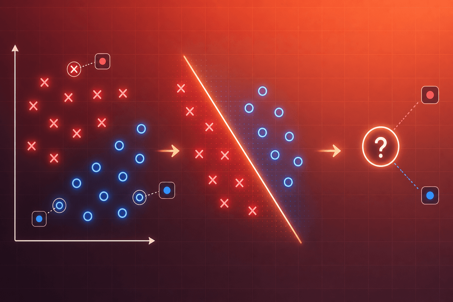
Supervised learning is the workhorse of applied machine learning: you have labeled examples (X, y) and want a model that predicts y from X. The core interview themes are (1) the bias-variance tradeoff, (2) choosing the right metric — accuracy is rarely what you actually want, (3) handling messy data (imbalance, leakage, scaling), and (4) knowing when to reach for a linear model, a tree ensemble, or a neural network.

This chapter walks through the interview-ready essentials, from evaluation to model choice. Read it top to bottom the first time, then use the Interview mode to test your recall and the Quiz to check yourself.

01

Fundamentals & theory

39 concepts

What is the bias-variance tradeoff?

easy
  • Bias is error from wrong assumptions (underfitting).
  • Variance is error from sensitivity to training data (overfitting).
  • Total generalization error decomposes as E[(yf^(x))2]=Bias[f^(x)]2+Var[f^(x)]+σ2\mathbb{E}\big[(y - \hat{f}(x))^{2}\big] = \mathrm{Bias}\big[\hat{f}(x)\big]^{2} + \mathrm{Var}\big[\hat{f}(x)\big] + \sigma^{2} where σ2\sigma^{2} is the irreducible noise.
  • You reduce bias with more complex models or better features, and reduce variance with more data, regularization, or ensembling.
  • The tradeoff means you can rarely minimize both at once.
Permalink

How do you detect and fix overfitting?

easy
  • Detect it when training loss keeps dropping but validation loss rises, or when train accuracy is much higher than validation.
  • Fixes: more data or augmentation, regularization (L1/L2, dropout), simpler model, early stopping, cross-validation, and ensembling.
  • In deep learning, add dropout, weight decay, and monitor the validation curve.
Permalink

What is k-fold cross-validation and when do you use stratified or grouped folds?

medium
  • Split the data into k folds; train on k-1 and validate on the held-out fold, then average.
  • Use stratified k-fold for classification (preserves class ratios per fold).
  • Use grouped k-fold when rows share an identity (same user, same patient) so the group never appears in both train and validation, preventing leakage.
  • Use time-series split for temporal data.
Permalink

Generative vs discriminative classifier — what's the difference?

medium
  • A discriminative model learns P(yx)P(y \mid x) directly (logistic regression, SVM, neural nets).
  • A generative model learns P(x, y) or P(xy)P(x \mid y) and applies Bayes' rule to get P(yx)P(y \mid x) (Naive Bayes, GDA, GANs, diffusion for x).
  • Discriminative models usually classify better; generative models can sample new data and often work with less data or missing features.
Permalink

What is the curse of dimensionality?

medium
  • As dimensions grow, data becomes sparse: distances between points concentrate, the volume needed to cover the space grows exponentially, and models that rely on locality (k-NN, kernel methods) degrade.
  • You need exponentially more data to maintain density.
  • Remedies: feature selection, dimensionality reduction (PCA, UMAP), regularization, and models that assume structure (trees, deep nets with inductive biases).
Permalink

Parametric vs non-parametric models — what's the difference?

easy
  • Parametric models have a fixed number of parameters that doesn't grow with the dataset (linear regression, logistic regression, GLMs, Naive Bayes).
  • They make strong assumptions about the functional form and are fast + data-efficient when those assumptions hold.
  • Non-parametric models grow in complexity with the data (KNN, decision trees, kernel methods, Gaussian processes).
  • They are more flexible but need more data and are prone to overfit.
Permalink

Why do we prefer simpler models when performance is equal?

easy
  • Occam's razor: among models with similar validation performance, the simpler one usually generalizes better and is cheaper to serve, easier to debug and monitor, and less prone to overfit noise.
  • Complexity should be justified by clear gains.
  • In practice this drives choices like linear over polynomial when residuals allow, smaller trees over deeper ones, and shallow ensembles over stacks-of-stacks.
Permalink

What does the no free lunch theorem say for ML?

medium
  • Averaged over all possible problems, no learning algorithm is better than random guessing.
  • Any advantage of an algorithm on one class of problems is offset by worse performance elsewhere.
  • Practically, this means model choice must match the structure of your data.
  • Trees dominate tabular data; CNNs dominate images; transformers dominate sequences — because their inductive biases match the domain, not because they are universally better.
Permalink

In one sentence, what is PAC learning?

hard
  • Probably Approximately Correct learning formalizes when a hypothesis class can be learned from a finite sample: for any small epsilon and delta, with enough samples the algorithm returns a hypothesis with error at most epsilon with probability at least 1-delta.
  • The required sample size scales with the complexity of the hypothesis class (VC dimension) and 1/epsilon.
Permalink

What is VC dimension and why should you care?

hard
  • The Vapnik-Chervonenkis dimension of a hypothesis class is the largest number of points it can shatter (label with any possible +/- assignment).
  • Higher VC dimension = more expressive class = higher risk of overfitting on small samples.
  • Linear classifiers in d dimensions have VC dim d+1.
  • VC bounds justify why you need more data as model capacity grows, and why regularization limits effective VC dim.
Permalink

What is Empirical Risk Minimization?

medium
  • ERM is the standard learning principle: pick the hypothesis in your class that minimizes the average loss on the training sample, as a proxy for the true (unknown) expected loss.
  • It works when the class is not too flexible relative to the sample size — otherwise you overfit.
  • Structural risk minimization adds a complexity penalty (regularization) to trade off training loss and capacity.
Permalink

Why do we care whether the loss landscape is convex?

medium
  • A convex loss (linear regression MSE, logistic regression log loss, SVM hinge, LASSO) has a single global minimum, so any local optimizer finds the best solution and results are reproducible.
  • Non-convex losses (neural networks, matrix factorization, deep boosting) have many local minima and saddle points — training is sensitive to initialization, learning rate, and stochasticity.
  • Convex problems admit strong theory (convergence, duality); non-convex ones rely on empirical tricks.
Permalink

What are the roles of the training, validation and test sets?

easy
  • Training set: fit the model parameters.
  • Validation set: tune hyperparameters, choose between models, early stop.
  • Test set: give one final unbiased estimate of generalization on unseen data.
  • If you touch the test set during model selection you leak information and overestimate performance.
  • Typical split for medium datasets: 70/15/15 or 60/20/20; for large data, ~1-2% is enough per set.
  • For small data use cross-validation on train+val and hold out a small test.
Permalink

What does the IID assumption mean and when is it violated?

medium
  • IID = samples are independent and identically distributed, drawn from the same population.
  • Standard ML theory (CV, generalization bounds, resampling) assumes IID.
  • It breaks with time series (temporal correlation), repeated measurements per subject, spatial data (autocorrelation), and streaming data where the distribution drifts.
  • Violations lead to over-optimistic error estimates; the fix is to use time-series splits, grouped CV, or drift-aware evaluation.
Permalink

Why is the base rate of the positive class critical to know?

medium
  • The base rate is the prior probability of the positive class in the population you'll deploy on.
  • It sets the floor for any metric — 99% accuracy is trivial on a 1%-positive problem by always predicting negative.
  • It affects PPV (precision) via Bayes rule even at fixed TPR/FPR.
  • Always report the class balance with your metrics and, when the deployment base rate differs from training, calibrate probabilities or adjust the decision threshold.
Permalink

What is inductive bias and why does every model have one?

medium
  • Inductive bias is the set of assumptions a learning algorithm uses to generalize from finite data to unseen examples.
  • Without an inductive bias, any function consistent with the training data is equally likely — no learning is possible.
  • Examples: linear regression assumes a linear conditional mean; CNNs assume locality and translation equivariance; trees assume axis-aligned splits; k-NN assumes locality in feature space.
  • Choosing a model = choosing an inductive bias that matches your data.
Permalink

What is the generalization gap and how do you shrink it?

medium
  • Generalization gap = expected test loss minus training loss.
  • A large gap means overfitting.
  • Shrink it with more data, stronger regularization (L2, dropout, weight decay), data augmentation, simpler models, ensembling, or early stopping.
  • It relates to the model's effective capacity and the sample size — the classic result is that gap decreases like sqrt(capacity / n).
Permalink

Why does OLS have a closed-form solution but logistic regression doesn't?

medium
  • OLS minimizes ||y - Xw||^2 which is quadratic in w — setting the gradient to zero yields the normal equations w  =  (XT  X)1w\; = \;(X^{T}\;X) - 1 XTX^{T} y, a closed form.
  • Logistic regression minimizes the log-loss which is convex but not quadratic (log of a sigmoid); its gradient has no closed-form root, so we solve it iteratively (IRLS, Newton, or SGD).
  • Both are convex, so the iterative solution reaches the unique optimum.
Permalink

What's the Bayesian interpretation of Ridge regression?

hard
  • Ridge regression is the maximum a posteriori (MAP) estimate under a Gaussian prior on the weights: w ~ N(0,  σ2/λ)N(0, \;\sigma^{2} / \lambda).
  • Equivalently, adding an L2 penalty on w is equivalent to assuming the coefficients are a priori small.
  • Lasso corresponds to a Laplace (double-exponential) prior on w, which has more probability mass at zero and heavier tails, explaining its sparsity behavior.
Permalink

What is a Generalized Linear Model and when is it the right tool?

medium
  • A GLM has three ingredients: (1) a linear predictor η=wx\eta = \mathbf{w}^{\top}\mathbf{x}; (2) a link function gg relating η\eta to E[yx]\mathbb{E}[y \mid x], so g(μ)=ηg(\mu) = \eta; (3) a distribution from the exponential family for yy (Gaussian → linear regression, Bernoulli → logistic, Poisson → Poisson regression, Gamma → Gamma regression).
  • Use a GLM when your target has a known non-Gaussian distribution but the mean-predictor relationship is approximately linear on the right scale.
Permalink

Why do we use cross-entropy (log loss) instead of MSE for classification?

medium
  • Cross-entropy matches the maximum-likelihood estimator for a Bernoulli / categorical target and has a well-shaped gradient when combined with sigmoid/softmax outputs — large errors give large gradients so the model learns fast.
  • MSE on top of sigmoid gives a very small gradient when predictions are confidently wrong (the sigmoid saturates), so training is slow and can get stuck.
  • Cross-entropy is also convex in the logits for logistic regression, MSE-with-sigmoid is not.
Permalink

How is logistic regression fit in practice?

medium
  • Two main approaches: (1) Iteratively Reweighted Least Squares (IRLS) — an implementation of Newton-Raphson on the log-likelihood.
  • Each iteration solves a weighted least squares problem with weights = p(1-p).
  • Converges in ~10-20 iterations for well-conditioned problems.
  • (2) First-order methods: L-BFGS, SAG, SAGA, SGD.
  • Better for large datasets and L1 penalty. scikit-learn uses 'lbfgs' by default; 'liblinear'/'saga' for L1.
Permalink

Your scikit-learn logistic regression warns 'lbfgs failed to converge'. What do you do?

medium
  • Common fixes: (1) standardize features — most convergence issues come from ill-scaled features; (2) increase maxiter\operatorname{max}_{\mathrm{iter}} (e.g., 1000); (3) increase regularization C down (stronger penalty smooths the loss); (4) switch solver ('saga' or 'liblinear' for L1, 'newton-cg' for very small data); (5) check for perfect / near-perfect separation and add L2 or drop the offending feature; (6) verify the target is not constant.
Permalink

How does Bayes' theorem drive Naive Bayes classification?

easy
  • For class c and features x, P(c    x)P(c\; \mid \;x)P(x    c)    P(c)P(x\; \mid \;c)\; \cdot \;P(c).
  • Naive Bayes assumes features are conditionally independent given the class: P(x    c)  =  prodjP(x\; \mid \;c)\; = \;\mathrm{prod}_{j} P(xj    c)P(x_{j}\; \mid \;c).
  • This lets you estimate each P(xj    c)P(x_{j}\; \mid \;c) separately (very fast, needs little data per parameter).
  • At prediction time you pick the class with the largest posterior score.
  • Priors P(c) are usually class frequencies; likelihoods P(xj    c)P(x_{j}\; \mid \;c) come from a chosen distribution (Gaussian, Multinomial, Bernoulli).
Permalink

The 'naive' independence assumption is almost always false. Why does Naive Bayes still work?

medium
  • Because classification only requires that the argmax over classes be correct — not that the posterior probabilities themselves be accurate.
  • Even when the independence assumption is violated, the decision boundary from NB can be close to optimal on many problems.
  • Its probabilities, however, are usually badly miscalibrated (too extreme, close to 0 or 1).
  • If you need calibrated probabilities, apply Platt or isotonic calibration on top.
Permalink

Why do we compute Naive Bayes scores in log space?

easy
  • The product prodj\mathrm{prod}_{j} P(xj    c)P(x_{j}\; \mid \;c) can be astronomically small (underflow) when there are many features (e.g., thousands of words in a document).
  • Taking logs turns the product into a sum: log P(c)  +  sumjP(c)\; + \;\mathrm{sum}_{j} log P(xj    c)P(x_{j}\; \mid \;c).
  • Sums are numerically stable, and the argmax is preserved because log is monotonic.
  • All practical NB implementations work in log space.
Permalink

What are the core assumptions behind Linear Discriminant Analysis (LDA)?

medium
  • LDA assumes each class-conditional distribution is Gaussian with class-specific mean but a *shared* covariance matrix Σ.
  • Under this assumption, the log-posterior is linear in x — the decision boundary between any two classes is a hyperplane.
  • It also assumes features are continuous.
  • When assumptions hold, LDA is close to Bayes-optimal and needs little data because it estimates fewer parameters than QDA (one Σ instead of one per class).
Permalink

Why does KNN degrade badly in high dimensions?

medium
  • In high dimensions, pairwise distances between random points concentrate — the ratio (max - min) / min distance approaches 0.
  • Every point becomes roughly the same distance from every other, so the concept of 'nearest' loses meaning and KNN votes become dominated by noise.
  • Remedies: apply dimensionality reduction (PCA, autoencoder) first, use domain-specific distance metrics, or switch to a model with stronger inductive bias (tree ensembles).
Permalink

How do KD-trees and ball-trees speed up KNN, and when do they stop helping?

medium
  • Both are spatial index structures that let you skip large portions of the training set during queries.
  • KD-trees split axis-aligned; efficient for low-dimensional data (~≤ 20 dims) with continuous features.
  • Ball-trees split with hyperspheres; better for non-Euclidean metrics and moderate dimensions.
  • Both degrade to brute force as dimensions grow (~50+), because the pruning becomes ineffective — then approximate methods (HNSW, FAISS, LSH) are the practical way to scale.
Permalink

Why not just fit a linear regression for a binary label (linear probability model)?

medium
  • You can — sometimes it even works reasonably as a quick baseline — but three problems bite in practice: (1) predicted probabilities aren't bounded to [0, 1]; (2) errors are heteroscedastic (variance = p(1-p) depends on x), so OLS standard errors are wrong; (3) it isn't the MLE for Bernoulli data.
  • Logistic regression fixes all three via the sigmoid link and the Bernoulli likelihood — that's why it's the default.
Permalink

What's the difference between probability, odds, and log-odds?

easy
  • Probability p in [0, 1].
  • Odds = p / (1 - p) in [0, ∞): 'how many times more likely than not'.
  • Log-odds (logit) = log(p / (1 - p)) in (-∞, ∞): a symmetric, unbounded scale, useful for modelling.
  • Logistic regression models the log-odds linearly in x, exactly because log-odds live on the real line (matching a linear predictor) and the inverse (sigmoid) automatically bounds probabilities to [0, 1].
Permalink

Why is a single decision tree considered a 'high-variance' model?

medium
  • A small change in the training data can produce a completely different tree: the first split cascades, so if a different feature is chosen at the top, everything below changes.
  • This makes individual trees unstable — predictions vary a lot with resampling.
  • Bagging (Random Forest) and boosting exploit this: averaging many independent (or corrected-residual) trees reduces variance dramatically without hurting bias.
Permalink

Why do decision trees (and boosted trees) fail to extrapolate?

medium
  • A tree predicts by returning the leaf value; leaves are bounded by the observed training range.
  • If a test feature is beyond the training range, the tree returns whatever leaf value corresponds to the closest region — no extrapolation.
  • This is fine on tabular data with stable distributions, but disastrous for time series with trend, or physics-style problems where extrapolation is the point.
  • Use linear models, splines, or neural nets when extrapolation matters.
Permalink

What is the out-of-bag (OOB) score in Random Forests?

medium
  • Each bootstrap sample leaves out ~37% of the training data (untouched by that tree).
  • For each training point x, aggregate predictions from the trees where x was NOT in-bag; compare to y.
  • This gives an internal estimate of generalization error at zero extra cost, roughly equivalent to a k-fold CV score, and lets you tune nestimatorsn_{\mathrm{estimators}} without a separate held-out set.
  • Enable with oobscore=True\mathrm{oob}_{\mathrm{score}} = \mathrm{True} in scikit-learn's RandomForestClassifier/Regressor.
Permalink

What is a support vector, and why does the SVM only depend on them?

medium
  • Support vectors are the training points that lie on the margin or inside it (or misclassified for soft margins) — points with non-zero Lagrange multipliers in the dual problem.
  • The optimal hyperplane is a linear combination of these support vectors alone: adding or removing non-SV points doesn't change the solution.
  • This makes SVMs memory-efficient at inference (store only SVs) and gives an implicit form of feature/data selection.
Permalink

Why don't kernel SVMs scale well to millions of samples?

medium
  • The dual problem has O(n2)O(n^{2}) memory (kernel matrix) and O(n2)O(n^{2}) to O(n3)O(n^{3}) training complexity.
  • For n = 1M, that's a trillion entries — impossible.
  • Workarounds: (1) linear SVM (LinearSVC / liblinear) which is O(nd) via primal optimization; (2) approximate kernels via random Fourier features / Nyström before feeding to a linear SVM; (3) switch entirely to gradient-boosted trees or neural nets, which routinely handle millions of samples.
Permalink

What is 'deviance' and why is it used to evaluate GLMs?

hard
  • Deviance = -2 * (log-likelihood of your model - log-likelihood of the saturated model).
  • Analog of squared error for non-Gaussian likelihoods: Poisson deviance for count data, Tweedie deviance for insurance-style claims, binomial deviance for logistic regression.
  • It's the natural loss for the corresponding GLM and gives coherent training + evaluation.
  • Modern GBM libraries expose Poisson / Tweedie / gamma deviance losses directly — pick the one matching your target distribution.
Permalink

You must pick ONE metric for your model. How do you decide?

medium
  • Start from the business objective, not the model: what does 'error' cost, and to whom?
  • Classification with asymmetric costs → expected cost or F-beta with the appropriate beta.
  • Rare-positive detection → PR-AUC / recall at fixed precision.
  • Ranking → NDCG or MAP.
  • Probabilistic forecasts → log loss or Brier + calibration.
  • Regression with tail-critical decisions → quantile loss.
  • Regression with symmetric costs and Gaussian errors → RMSE.
  • Always report multiple metrics; the *primary* one is the one you optimize and stop-arg on.
Permalink

An interviewer asks you to build a churn model. What do you do before touching any algorithm?

easy
  • Define the prediction problem precisely: what counts as churn, and over what horizon.
  • Fix the prediction time, so every feature is something you would actually have at that moment.
  • Then build the dumbest possible baseline: predict the base rate, or a single rule like 'no login in 30 days'.
  • That baseline is what every later model must beat, and it takes an hour instead of a week.
  • Only then pick a model family, and prefer gradient boosting on tabular data.
  • Candidates who jump straight to model choice usually end up with leakage or a target that nobody agreed on.
Permalink
02

Linear & regularized regression

35 concepts

L1 vs L2 regularization — what's the difference?

easy
  • L2 (ridge) adds sum(w2)\mathrm{sum}(w^{2}) to the loss and shrinks weights smoothly toward zero.
  • L1 (lasso) adds sum(w)\mathrm{sum}( \mid w \mid ) and pushes weights exactly to zero, giving sparse solutions and doing feature selection.
  • Elastic Net combines both.
  • Use L1 when you want a sparse, interpretable model; use L2 when you want smooth shrinkage and stable coefficients.
Permalink

Why is logistic regression called a linear model if it uses a sigmoid?

medium
  • The decision boundary is linear in the input features because the model is linear in the log-odds: logit(p)  =  wT\mathrm{logit}(p)\; = \;w^{T} x + b.
  • The sigmoid only maps that linear score into [0, 1] for a probability.
  • So the model is linear in parameters and features; only the link function is nonlinear.
Permalink

What are the classical assumptions of linear regression?

medium
  • (1) Linearity: the conditional mean E[yx]E[y \mid x] is linear in the parameters.
  • (2) Independence of errors.
  • (3) Homoscedasticity: constant error variance across x.
  • (4) Normality of errors (needed for exact inference on coefficients, not for point estimates).
  • (5) No perfect multicollinearity between features.
  • Violations don't ruin prediction but do ruin confidence intervals, p-values, and standard errors.
Permalink

How do you interpret a coefficient in a multiple linear regression?

easy
  • The coefficient βj\beta_{j} is the expected change in y per one-unit increase in xjx_{j} while holding all other features fixed — the partial or ceteris-paribus effect.
  • Sign gives the direction; magnitude depends on the scale of xjx_{j}.
  • If features are standardized, |βj  is\beta_{j} \mid \;\mathrm{is} comparable across features (standardized beta / beta weight).
  • Careful: 'holding others fixed' only makes sense if features are not perfectly collinear.
Permalink

What is VIF and when do you worry about multicollinearity?

medium
  • Variance Inflation Factor of feature xj  =  1  /  (1    Rj2)x_{j}\; = \;1\; / \;(1\; - \;R_{j}^{2}), where Rj2R_{j}^{2} is the R2R^{2} of regressing xjx_{j} on the other features.
  • VIF = 1 means no collinearity; VIF > 5 or 10 is a common warning threshold.
  • High VIF inflates coefficient standard errors, makes individual coefficients unstable and hard to interpret, but doesn't harm overall prediction.
  • Fixes: drop redundant features, combine them (PCA), or use ridge regression which is stable under collinearity.
Permalink

How do you handle strong multicollinearity in a linear model?

medium
  • (1) Drop one of the correlated features (highest VIF first).
  • (2) Combine them via PCA or domain-driven aggregation.
  • (3) Switch to Ridge regression — the L2 penalty stabilizes coefficients under collinearity by shrinking correlated features together.
  • (4) Collect more data if the collinearity is sample-specific.
  • Note: multicollinearity does not bias predictions, only inference on individual coefficients, so if you only need predictions you can leave it alone.
Permalink

How do you detect and fix heteroscedasticity?

hard
  • Heteroscedasticity = error variance depends on x.
  • Detect with a residuals-vs-fitted plot (funnel shape), Breusch-Pagan or White test.
  • Consequences: OLS coefficients remain unbiased but standard errors are wrong, so t-tests and CIs are invalid.
  • Fixes: (1) transform y (log, sqrt, Box-Cox) if variance increases with the mean; (2) use weighted least squares with weights proportional to 1/variance; (3) use heteroscedasticity-robust (sandwich / White) standard errors.
Permalink

Adding a feature raised R2R^2. Does that mean the model improved?

easy
  • R2=1SSresSStotR^{2} = 1 - \frac{SS_{\mathrm{res}}}{SS_{\mathrm{tot}}} is the fraction of variance explained; it never decreases when you add a feature, even a useless one.
  • Adjusted R2R^{2} penalizes for the number of features and can decrease when you add a feature that doesn't help.
  • Use adjusted R2R^{2} for model comparison across different feature counts; use R2R^{2} to describe fit at a fixed feature set.
  • Both can be misleading for non-linear models; prefer AIC/BIC or CV.
Permalink

Can R2R^{2} be negative? What does that mean?

medium
  • Yes. R2=1SSresSStotR^{2} = 1 - \frac{SS_{\mathrm{res}}}{SS_{\mathrm{tot}}} compares your model's residual sum of squares to that of a constant-mean baseline.
  • A negative R2R^{2} on a test set means your model is worse than predicting the mean everywhere — usually a sign of severe overfitting or distribution shift.
  • On the training set with intercept, R2R^{2} is always in [0,1][0, 1]; the negative case only appears on held-out data or intercept-free fits.
Permalink

When would you use robust regression (Huber, RANSAC) instead of OLS?

medium
  • Use robust regression when the data contains outliers that shouldn't dominate the fit.
  • OLS minimizes squared error, so a single large-residual point can pull the line dramatically.
  • Huber loss is quadratic near zero and linear in the tails, giving less weight to outliers.
  • RANSAC fits on random subsets and picks the fit with the most inliers — great when up to ~50% of points are contaminated.
  • Quantile regression is another robust option that models a specific quantile.
Permalink

What's the main risk of polynomial regression?

easy
  • High-degree polynomial features overfit dramatically: they can hit training points exactly while oscillating wildly between them (Runge's phenomenon).
  • Predictions extrapolate very poorly outside the training range.
  • Alternatives: use splines (piecewise low-degree polynomials with continuity), local polynomials (LOESS), regularized polynomials, or non-parametric models like trees.
  • If you must use polynomials, standardize inputs and combine with L2 regularization.
Permalink

When should you add interaction features to a linear model?

medium
  • Add xi    xjx_{i}\; \cdot \;x_{j} when the effect of one feature on y depends on the value of another and your model class can't discover this on its own (linear models can't).
  • Common in marketing (channel × segment), medicine (treatment × age), and pricing (product × geography).
  • Signs: residual patterns when you slice by a second feature, domain knowledge of moderation, or when a tree model beats a linear model but you want linear interpretability.
Permalink

When does log-transforming the target help a regression model?

medium
  • Log-transform y when (1) y is strictly positive and right-skewed (revenue, counts, biological measurements, house prices), (2) residuals show heteroscedasticity that shrinks after the transform, (3) you care about relative rather than absolute errors — modeling log(y)\operatorname{log}(y) is equivalent to modeling percentage errors.
  • Watch out: predictions in log space need exp()\operatorname{exp}() to be brought back, and the expectation is biased (E[exp(z)]    exp(E[z]))(E[\operatorname{exp}(z)]\; \ne \;\operatorname{exp}(E[z])).
Permalink

What do Box-Cox and Yeo-Johnson transforms do?

medium
  • Both are power transforms that find a lambda making the data approximately Gaussian and stabilizing variance.
  • Box-Cox requires strictly positive data.
  • Yeo-Johnson generalizes to any real values (including zero and negatives).
  • They're useful for the target of a regression or heavily skewed features feeding a linear/Gaussian-based model.
  • Not needed for tree ensembles (monotone-invariant) or for deep nets (BatchNorm handles it).
Permalink

Why does Ridge regression give more stable coefficients than OLS?

medium
  • Ridge solves (XT  X  +  λ  I)(X^{T}\;X\; + \;\lambda\;I) w  =  XTw\; = \;X^{T} y instead of XTX^{T} X w  =  XTw\; = \;X^{T} y.
  • Adding lambda I to the diagonal keeps the matrix invertible even when features are collinear or when p > n, and shrinks coefficients toward zero proportionally to their scale.
  • The shrinkage introduces bias but drastically reduces variance — often a favourable tradeoff for prediction.
  • Ridge does not zero-out coefficients, it just makes them small and stable.
Permalink

Why does L1 (Lasso) produce sparse coefficients but L2 (Ridge) does not?

medium
  • Geometrically, the L1 constraint region is a diamond with corners on the axes, so the loss contour tends to intersect the constraint at a corner where some coefficients are exactly zero.
  • The L2 region is a sphere, so intersections are typically off-axis — coefficients become small but not zero.
  • Algebraically, L1's subgradient at zero is a range containing zero, so a solver can 'stick' coefficients at exactly zero.
Permalink

When is Elastic Net better than pure Lasso or Ridge?

medium
  • Elastic Net combines L1 and L2 penalties: α    (ρ    w1  +  (1ρ)    0.5    w22)\alpha\; \cdot \;(\rho\; \cdot \; \mid w \mid 1\; + \;(1 - \rho)\; \cdot \;0.5\; \cdot \; \mid w \mid 2^{2}).
  • Use it when (1) features are highly correlated — Lasso arbitrarily picks one and drops the rest, Elastic Net groups correlated features together via the L2 term; (2) you have more features than samples (p >> n) — Lasso caps the number of selected features at n.
  • Tune rho on validation data.
Permalink

How do you choose the regularization strength (lambda / alpha)?

medium
  • Cross-validation over a log-spaced grid is the standard approach — pick alpha minimizing average validation loss.
  • Coefficient path plots (coefficient vs log alpha) help understand which features enter/exit at what strength.
  • For efficiency, use algorithms that compute the whole path (LARS, coordinate descent with warm starts): scikit-learn's LassoCV / RidgeCV / ElasticNetCV do this out of the box.
  • Standardize features first; alpha's meaningful scale depends on it.
Permalink

Why must you standardize features before applying L1 or L2 regularization?

easy
  • The penalty is applied uniformly to all coefficients, but the natural scale of a coefficient depends on the scale of its feature (weight * feature = signal).
  • Without standardization, a feature measured in millimetres would get a huge coefficient and be over-penalized versus one in metres.
  • Standardizing (mean 0, std 1) puts coefficients on comparable scales, so alpha has a consistent effect and coefficient magnitudes become interpretable.
Permalink

In one sentence, what does the LARS algorithm compute?

hard
  • Least Angle Regression is a stagewise algorithm that computes the entire regularization path of Lasso coefficients (from full L1 penalty down to zero penalty) in about the same cost as one OLS fit, by adding features to the active set in the order of highest correlation with the current residual and moving in a direction equiangular to them.
Permalink

When would you use Group Lasso instead of standard Lasso?

hard
  • Group Lasso applies an L2 penalty within groups of coefficients and an L1 penalty across groups: entire groups get selected or dropped together.
  • Use it when features come in natural groups — one-hot dummies of a categorical variable, spline basis functions, features from the same sensor.
  • Standard Lasso would drop some dummies of a category, which is semantically odd; Group Lasso keeps or drops the whole category.
Permalink

When is quantile regression more useful than mean (OLS) regression?

hard
  • Quantile regression models a specific conditional quantile of y (e.g., the median, 90th percentile) instead of the mean.
  • Use it when (1) you care about tails, not the average — delivery time SLA, inventory sizing, risk quantiles; (2) the target distribution is asymmetric or heavy-tailed; (3) you want a prediction interval by fitting several quantiles.
  • It minimizes the pinball (quantile) loss instead of MSE.
Permalink

What is 'perfect separation' in logistic regression and how do you fix it?

hard
  • Perfect separation happens when a feature (or combination) fully separates the classes: the MLE for the corresponding weight goes to +/- infinity and the solver never converges (or gives massive coefficients with huge standard errors).
  • Fixes: (1) add L2 regularization (drives the weight to a finite value); (2) use Firth's penalized likelihood; (3) drop or bin the separating feature.
  • Common on tiny or heavily imbalanced datasets and one-hot rare categories.
Permalink

L1 vs L2 in logistic regression — practical differences.

easy
  • Same intuition as in linear regression: L2 (default) shrinks all coefficients smoothly and stabilizes training under multicollinearity; L1 produces sparse coefficients and performs feature selection during training.
  • In scikit-learn, use penalty='l1' with the 'liblinear' or 'saga' solver.
  • L1 is nice for interpretable, sparse models on wide (many-feature) data; L2 is the default for prediction accuracy.
  • Elastic-Net penalty combines both.
Permalink

What is Laplace (additive) smoothing in Naive Bayes?

easy
  • It adds a small constant alpha to every count when estimating P(xj    c)P(x_{j}\; \mid \;c) so no probability is ever exactly zero.
  • Without smoothing, a single word never seen with class c in training would give P(document    c)  =  0P(\mathrm{document}\; \mid \;c)\; = \;0, killing the posterior.
  • Alpha=1 is Laplace smoothing; smaller alpha (e.g., 0.01) is Lidstone smoothing.
  • Choose it by cross-validation — it plays the role of a regularizer for the likelihood.
Permalink

Pre-pruning vs post-pruning in decision trees — what's the difference and when do you use each?

medium
  • Pre-pruning stops the tree from growing during construction, via maxdepth\operatorname{max}_{\mathrm{depth}}, minsamplessplit\operatorname{min}_{\mathrm{samples}}\mathrm{split}, minsamplesleaf\operatorname{min}_{\mathrm{samples}}\mathrm{leaf}, or minimpuritydecrease\operatorname{min}_{\mathrm{impurity}}\mathrm{decrease}.
  • Fast and simple but you may stop too early (horizon effect).
  • Post-pruning (cost-complexity or reduced-error pruning) grows the tree fully then removes subtrees using a held-out set or a complexity penalty.
  • Usually gives a slightly better bias-variance tradeoff but requires the extra pass.
  • Modern ensembles (RF, GBM) rely on pre-pruning + averaging, which is why deep individual trees are OK in them.
Permalink

How does cost-complexity (CCP) pruning work?

hard
  • Grow the tree fully.
  • Define Rα(T)  =  R(T)  +  αR_{\alpha}(T)\; = \;R(T)\; + \;\alpha * |T|, where R(T) is the training error, |T  isT \mid \;\mathrm{is} the number of leaves, and alpha ≥ 0 penalizes complexity.
  • For each alpha, the subtree minimizing RαR_{\alpha} is unique and nested — you get a full sequence of subtrees indexed by alpha.
  • Pick alpha via cross-validation on the sequence.
  • Scikit-learn exposes it via costcomplexitypruning\mathrm{cost}_{\mathrm{complexity}}\mathrm{pruning}_path and the ccpα\mathrm{ccp}_{\alpha} argument.
Permalink

How does early stopping work in gradient boosting and why is it important?

easy
  • Monitor validation loss after each tree is added; stop when it hasn't improved for earlystoppingrounds\mathrm{early}_{\mathrm{stopping}}\mathrm{rounds} boosting iterations.
  • Returns the model at the best iteration (not the last).
  • Effect: automatic selection of nestimatorsn_{\mathrm{estimators}}, protection against overfitting, faster training when convergence happens early.
  • Set nestimatorsn_{\mathrm{estimators}} very large (2000+) and let early stopping pick the actual count.
  • Requires an evalset  /  validationdata\mathrm{eval}_{\mathrm{set}}\; / \;\mathrm{validation}_{\mathrm{data}} — never use the test set for this.
Permalink

How does the C parameter in an SVM affect the fit?

medium
  • C weights the misclassification penalty in the soft-margin loss (opposite of a typical regularization strength — larger C means less regularization).
  • Large C: try hard to classify every training point correctly → narrow margin, complex boundary, high variance.
  • Small C: tolerate more margin violations → wider margin, simpler boundary, high bias.
  • Tune C on a log-spaced grid with CV.
  • With an RBF kernel, C interacts with gamma — tune them jointly.
Permalink

How does SVM adapt to regression (SVR)?

medium
  • SVR uses an epsilon-insensitive loss: residuals with  y    yhat\mathrm{with}\; \mid y\; - \;y_{\mathrm{hat}}| ≤ epsilon are free (zero penalty), residuals outside are penalized linearly (like L1).
  • Combined with the kernel trick, it fits a flexible non-linear function using only a subset of training points as support vectors.
  • Tune C (violation penalty), epsilon (tube width), and gamma (for RBF).
  • Works well on small/medium tabular problems where linear methods underfit and boosted trees are overkill.
Permalink

What is Huber loss and why is it a compromise between MAE and MSE?

medium
  • Huber loss is quadratic for  r\mathrm{for}\; \mid r| ≤ delta (like MSE) and linear beyond delta (like MAE), joined smoothly at delta.
  • Combines MSE's differentiability near zero (good gradients for optimization) with MAE's robustness to outliers (linear tail doesn't blow up on rare huge errors). delta acts as an outlier threshold — typical values are 1    σy1\; \cdot \;\sigma_{y} or set via CV.
  • Used in robust regression, Huber-loss neural nets, and reinforcement learning (Huber for value updates).
Permalink

What does the quantile (pinball) loss measure?

hard
  • For quantile tau in (0, 1), pinball loss(r) = tau * r if r > 0 else (tau - 1) * r, where r  =  y    yhatr\; = \;y\; - \;y_{\mathrm{hat}}.
  • Minimizing it fits the conditional tau-quantile of y given x. τ  =  0.5\tau\; = \;0.5 → median (equivalent to MAE). τ  =  0.9\tau\; = \;0.9 → 90th percentile prediction — great for delivery-time SLAs, inventory sizing, risk quantiles.
  • Fit multiple quantiles to construct prediction intervals: e.g., 0.05 and 0.95 give a 90% interval.
  • Used by quantile regression, LightGBM's quantile objective, and neural nets with pinball loss.
Permalink

What is stability selection?

hard
  • Run your feature-selection method (usually Lasso) on many random subsamples of the data.
  • Record how often each feature is selected.
  • Keep only features selected in ≥ πthr\pi_{\mathrm{thr}} (typically 60-90%) of subsamples.
  • Rationale: any single Lasso fit is unstable — features come and go with the sample.
  • Stability selection isolates features that are robustly informative across data resamples, with theoretical false-discovery-rate guarantees.
Permalink

What are monotonic constraints in gradient boosting and when are they worth using?

hard
  • They force the predicted output to move in one direction as a feature increases.
  • Useful when domain knowledge is certain: risk should not fall as debt rises, and price should not fall as square footage rises.
  • Benefits are regulatory defensibility, more stable behaviour in sparse regions of the feature space, and mild regularization that often helps on small data.
  • Cost is bias if the true relationship is not monotone, so check that the constraint does not degrade validation performance.
  • Supported directly in XGBoost, LightGBM and CatBoost.
Permalink

When would you use quantile regression instead of predicting the mean?

medium
  • When the decision needs a range rather than a point.
  • Inventory planning cares about the 90th percentile of demand, not the average, because stocking to the mean stocks out half the time.
  • Delivery estimates quote a pessimistic quantile so most promises are kept.
  • Quantile regression minimizes the pinball loss, which weights under- and over-prediction asymmetrically, and gives you an interval by fitting several quantiles.
  • It is also robust to outliers, since the median is not pulled by extreme values the way the mean is.
  • Available natively in LightGBM and scikit-learn.
Permalink
03

Logistic regression & classification basics

29 concepts

Precision vs recall — when do you optimize each?

easy
  • Precision = TP / (TP + FP): of the items flagged positive, how many really are.
  • Recall = TP / (TP + FN): of the actual positives, how many we caught.
  • Optimize precision when false positives are costly (spam filter, fraud alert to a user).
  • Optimize recall when missing a positive is costly (cancer screening, security threats).
  • F1 balances them.
Permalink

How do you read a confusion matrix and derive the key metrics?

easy
  • Rows = actual class, columns = predicted class (or vice versa).
  • Cells: TP, FP, TN, FN.
  • Accuracy = (TP+TN)/all.
  • Precision = TP/(TP+FP).
  • Recall = TP/(TP+FN).
  • Specificity = TN/(TN+FP).
  • F1 = 2·P·R/(P+R).
  • Read it to see which class the model confuses with which — a diagonal-heavy matrix means good separation.
Permalink

One-vs-Rest, One-vs-One, and softmax — how do you choose for multi-class?

medium
  • One-vs-Rest trains K binary classifiers (class k vs the rest); simple and calibrates per-class, but scores aren't jointly normalized.
  • One-vs-One trains K(K-1)/2 binary models between every pair; more models but each sees a balanced binary problem, useful for SVMs. Softmax / multinomial logistic regression jointly models all classes with a single objective; the natural choice for logistic regression and neural nets and it produces coherent probabilities that sum to one.
Permalink

Write out the softmax function and its main property.

easy
  • softmax(z)k  =  exp(zk)  /  sumj\operatorname{softmax}(z)k\; = \;\operatorname{exp}(z_{k})\; / \;\mathrm{sum}_{j} exp(zj)\operatorname{exp}(z_{j}).
  • It maps a vector of real logits to a probability distribution: values in (0, 1) that sum to 1.
  • It's invariant to adding a constant to all logits (that's why we subtract max(z) for numerical stability).
  • The winner is the argmax; adjacent logits produce similar probabilities so the mapping is smooth and differentiable — perfect for gradient descent.
Permalink

How do you interpret a logistic regression coefficient as an odds ratio?

medium
  • In log(odds)  =  wT\operatorname{log}(\mathrm{odds})\; = \;w^{T} x, a one-unit increase in xjx_{j} multiplies the odds by exp(wj)\operatorname{exp}(w_{j}). exp(wj)\operatorname{exp}(w_{j}) is the odds ratio: 1.5 means a 50% relative increase in odds per unit of xjx_{j}.
  • Positive w    oddsw\; \to \;\mathrm{odds} ratio  >  1    outcome\mathrm{ratio}\; > \;1\; \to \;\mathrm{outcome} more likely; negative w -> < 1    less1\; \to \;\mathrm{less} likely.
  • For a categorical predictor with a reference level, exp(w)\operatorname{exp}(w) is the odds ratio between that category and the reference.
Permalink

How do class weights work in logistic regression, and when do you use them?

medium
  • Class weights re-weight the log-loss contributions of each class so the minority class carries more penalty when misclassified.
  • 'balanced' in scikit-learn sets weightc  =  nsamples  /  (nclasses    nc)\mathrm{weight}_{c}\; = \;n_{\mathrm{samples}}\; / \;(n_{\mathrm{classes}}\; \cdot \;n_{c}).
  • Effect: pushes the decision boundary toward the majority class and improves recall on the minority class, at the cost of precision.
  • Use when the positive class is rare and false negatives are more costly than false positives.
Permalink

'multinomial' vs 'ovr' setting in scikit-learn's LogisticRegression — what changes?

medium
  • 'multinomial' fits a joint softmax model over all K classes with a single log-loss objective — the natural probabilistic model for multi-class.
  • 'ovr' trains K independent binary logistic regressions (class k vs the rest) and normalizes per-example at prediction time.
  • Multinomial usually gives better-calibrated probabilities and slightly better accuracy; OvR is simpler and lets you look at per-class binary models but doesn't guarantee coherent probabilities.
Permalink

Gaussian NB vs Multinomial NB vs Bernoulli NB — when do you use each?

medium
  • Gaussian NB: continuous features assumed to be normally distributed per class (baseline for tabular numeric data).
  • Multinomial NB: counts / term frequencies — the go-to for bag-of-words text classification.
  • Bernoulli NB: binary indicators — text with presence/absence of terms, or clickstream flags.
  • Complement NB is a Multinomial NB variant that's more robust on imbalanced text corpora.
Permalink

When would LDA outperform logistic regression?

hard
  • When (1) classes are approximately Gaussian with similar covariances — LDA is the maximum-likelihood classifier for that model, more efficient than logistic regression which is agnostic to the feature distribution; (2) the training set is small — LDA has fewer parameters and estimates them from all of the data at once; (3) classes are well-separated — logistic regression can suffer from perfect separation, LDA doesn't.
  • Logistic regression usually wins when features are non-Gaussian or highly correlated.
Permalink

What is the nearest centroid (Rocchio) classifier and when is it useful?

easy
  • Compute the mean feature vector per class; classify a new point as the class whose centroid is closest (usually Euclidean or cosine).
  • Extremely simple, no hyperparameters, very fast, no training beyond averaging.
  • Works well when classes are roughly spherical and well-separated in feature space.
  • Good baseline for text classification with TF-IDF (called Rocchio's method).
  • Fails when class distributions are non-spherical or overlapping.
Permalink

How does temperature scaling calibrate a classifier's probabilities?

medium
  • You take the trained logits z, divide by a scalar T > 0, then softmax: p = softmax(z / T).
  • T is fit on a held-out validation set by minimizing NLL.
  • T > 1 sharpens toward uniform (softens overconfident predictions — the typical case for deep nets); T < 1 sharpens toward one-hot.
  • It changes only confidence, not the argmax, so accuracy is unchanged but calibration (ECE, Brier) improves.
  • Cheap, single-parameter, widely used for post-hoc calibration.
Permalink

Why is accuracy a bad primary metric for many real-world problems?

easy
  • Accuracy weights every error equally and ignores class balance.
  • On a 99% negative dataset, always predicting negative gives 99% accuracy — a model that's completely useless.
  • Even on balanced problems it hides asymmetric costs (missed fraud is worse than a false alarm, or vice versa).
  • Prefer metrics matched to the deployment cost: precision at fixed recall, F1, PR-AUC, expected cost, Brier score.
  • Always report accuracy alongside the class prior so readers can spot base-rate issues.
Permalink

What is F-beta score and when is F1 not enough?

medium
  • Fβ  =  (1  +  β2)    P    R  /  (β2    P  +  R)F_{\beta}\; = \;(1\; + \;\beta^{2})\; \cdot \;P\; \cdot \;R\; / \;(\beta^{2}\; \cdot \;P\; + \;R) generalizes F1 with a weight on recall vs precision. β  =  1\beta\; = \;1 → F1 (equal). β  =  2\beta\; = \;2 (F2) → recall matters 4x more than precision — appropriate for medical screening where missing positives is very costly. β  =  0.5\beta\; = \;0.5 (F0.5) → precision matters 4x more — for a spam filter where false positives annoy users.
  • F1's implicit assumption is that precision and recall are equally important — often they aren't.
Permalink

Macro vs micro vs weighted averaging in multi-class metrics — how do you choose?

medium
  • Macro: compute metric per class, then average with equal weight.
  • Treats each class equally — useful when small classes matter (e.g., rare diseases).
  • Micro: aggregate TP/FP/FN across all classes then compute the metric globally.
  • Dominated by frequent classes; equals accuracy for single-label problems.
  • Weighted: per-class metric weighted by class support.
  • Compromise between macro and micro.
  • Rule of thumb: report macro when classes have unequal importance; micro/weighted when the aggregate is the target.
Permalink

What is Cohen's kappa and why is it useful?

medium
  • Cohen's κ  =  (po    pe)  /  (1    pe)\kappa\; = \;(p_{o}\; - \;p_{e})\; / \;(1\; - \;p_{e}), where pop_{o} is observed agreement (accuracy) and pep_{e} is the agreement expected by chance given class marginals.
  • It corrects accuracy for the baseline of random guessing given the class prior.
  • Range: [-1, 1]. 0 = no better than chance; 1 = perfect.
  • Rules of thumb: 0.2 slight, 0.4 fair, 0.6 substantial, 0.8+ almost perfect.
  • Useful for imbalanced classification and inter-annotator agreement.
Permalink

What is the Matthews Correlation Coefficient (MCC) and when should you use it?

medium
  • MCC = (TP*TN - FP*FN) / sqrt((TP+FP)(TP+FN)(TN+FP)(TN+FN)) — the Pearson correlation coefficient between predicted and true binary labels.
  • Range [-1, 1]: 1 perfect, 0 chance, -1 perfectly wrong.
  • Its advantage over F1: symmetric in positive and negative classes (F1 ignores TN), so it's a fair single-number summary even on imbalanced data.
  • Great for reporting binary classifier quality in one number.
Permalink

What is log loss (cross-entropy) and what does a specific value mean?

medium
  • For binary: log loss = -1/n * sum [y log(p) + (1-y) log(1-p)].
  • It's the negative log-likelihood of the observed labels under the predicted probabilities — proper scoring rule that rewards well-calibrated confident predictions and heavily punishes confident mistakes. log(0.5)\operatorname{log}(0.5) ≈ 0.693 is the loss of always predicting 0.5 (max-uncertainty baseline).
  • Above that, your model is worse than uninformative; below, it's actually learning something.
  • Never use log loss for evaluation on a mis-calibrated model.
Permalink

What is the Brier score and how does it compare to log loss?

medium
  • Brier = 1/n * sum (pi    yi)2(p_{i}\; - \;y_{i})2 — mean squared error between predicted probability and true label.
  • Range [0, 1] for binary.
  • Like log loss, it's a proper scoring rule that penalizes miscalibration.
  • Differences: Brier is bounded and quadratic (less punishing on confident mistakes than log loss), decomposable into calibration + refinement + uncertainty terms (Murphy decomposition), and interpretable in probability units.
  • Prefer Brier when confident misprediction shouldn't dominate the metric.
Permalink

What is top-k accuracy and when do you use it?

easy
  • Top-k counts a prediction as correct if the true class is among the top-k predicted classes ranked by score.
  • Common in image classification with many classes (ImageNet top-5), recommender systems (was the right item in the top-10 recommendations?), and retrieval-style tasks.
  • Top-k relaxes the single-choice requirement — appropriate when downstream UX shows multiple candidates.
  • Report both top-1 and top-k for calibration between raw and forgiving evaluation.
Permalink

What is balanced accuracy?

easy
  • Balanced accuracy = (sensitivity + specificity) / 2 for binary, or the macro average of per-class recall for multi-class.
  • It corrects accuracy by treating every class equally regardless of size — a 50% baseline for random guessing on any class balance.
  • Handy single-number summary for imbalanced classification; equivalent to accuracy on perfectly balanced data.
  • Doesn't use precision, so pair it with PR-AUC when the positive class is what you care about.
Permalink

What is the geometric mean (G-mean) in classification metrics?

medium
  • G-mean = sqrt(sensitivity * specificity).
  • Only high when both true positive and true negative rates are high — a single point going to zero drags the metric to zero.
  • Useful for imbalanced problems where you want a classifier that performs well on both classes, not one that trivially favors the majority.
  • Common in medical diagnostics.
Permalink

What is Youden's J statistic and how is it used?

medium
  • J = sensitivity + specificity - 1.
  • It's the vertical distance from the ROC curve to the diagonal at a given operating point.
  • The threshold that maximizes J is the 'Youden optimal' operating point — often used in medical statistics to pick a screening cutoff that balances sensitivity and specificity.
  • Assumes equal cost of FP and FN — use cost-weighted variants when they differ.
Permalink

How do you interpret an ROC curve, and what point matters?

medium
  • ROC plots True Positive Rate (sensitivity) vs False Positive Rate (1 - specificity) as the decision threshold sweeps from 1 to 0.
  • The diagonal is random guessing; the top-left corner is perfect.
  • AUC is the area under it — the probability that a random positive is scored higher than a random negative.
  • The 'best' operating point depends on cost: often top-left-most, or the intersection with an iso-cost line matching your FP/FN penalties.
Permalink

What does ROC-AUC really measure, and what's a good value?

easy
  • AUC is the probability that a random positive example is scored higher than a random negative example (equivalent to the Mann-Whitney U statistic normalized). 0.5 = random; 1.0 = perfect ranking.
  • Rules of thumb: 0.7 acceptable, 0.8 good, 0.9+ excellent.
  • Beware: an AUC in isolation says nothing about calibration or the actual decision threshold — a classifier can have high AUC and still make horrible probability estimates.
Permalink

What are the main pitfalls of relying on ROC-AUC?

medium
  • (1) On heavily imbalanced data, ROC-AUC is optimistic because the false positive rate is dominated by a huge number of negatives — PR-AUC is more informative.
  • (2) AUC is threshold-independent — a model with great AUC can still have terrible precision at any usable threshold.
  • (3) It doesn't reward calibration — two models with identical AUC can have very different probability quality.
  • (4) Comparing AUC across datasets with different class balances is misleading.
  • Always pair AUC with a calibration metric and a cost-aware operating point.
Permalink

How do you select the decision threshold for a binary classifier?

medium
  • Compute predicted probabilities on validation, then choose the threshold based on your business objective: (a) maximize F1 → argmax over t of F1(y, p > t); (b) fixed recall → smallest t with recall ≥ target, maximizing precision; (c) expected cost → t that minimizes FPcostFP  +  FNcostFN\mathrm{FP}_{\mathrm{cost}} \cdot \mathrm{FP}\; + \;\mathrm{FN}_{\mathrm{cost}} \cdot \mathrm{FN}.
  • Never tune threshold on the test set.
  • If probabilities are poorly calibrated, calibrate first, then threshold.
  • Threshold tuning is often more impactful than model choice.
Permalink

How do you evaluate a multi-label classifier?

medium
  • Common metrics: (a) Hamming loss = fraction of misclassified labels (per-label error) — lenient; (b) exact match / subset accuracy = fraction of examples where ALL labels are correctly predicted — strict; (c) per-label F1 with macro/micro averaging — the workhorse; (d) label ranking metrics (mean average precision, coverage error) when scores matter more than binary decisions.
  • Always report per-label metrics too, especially when label frequencies differ.
Permalink

MAP, NDCG, MRR — when do you use each in ranking?

hard
  • MRR (Mean Reciprocal Rank): 1/rank of the first relevant item, averaged over queries.
  • Ideal for 'find one right answer' tasks.
  • MAP (Mean Average Precision): mean of per-query average precision — for tasks with multiple relevant items and only binary relevance.
  • NDCG (Normalized Discounted Cumulative Gain): uses graded relevance and log-position discount — the standard for search / recommendation ranking with graded labels.
  • Use MRR for factoid QA, MAP for binary relevance, NDCG for graded relevance.
Permalink

How do you evaluate a classifier when FP and FN have different costs?

hard
  • Assign explicit costs CFPC_{\mathrm{FP}} and CFNC_{\mathrm{FN}}.
  • Compute expected cost per example  =  CFP    FPR    P(neg)  +  CFN    FNR    P(pos)\mathrm{example}\; = \;C_{\mathrm{FP}}\; \cdot \;\mathrm{FPR}\; \cdot \;P(\mathrm{neg})\; + \;C_{\mathrm{FN}}\; \cdot \;\mathrm{FNR}\; \cdot \;P(\mathrm{pos}).
  • Pick the threshold that minimizes it on validation.
  • Report expected loss in dollar / operational units, not just precision-recall.
  • If costs are unknown but ordinal (FN worse than FP), use ROC iso-cost lines: parallel lines whose slope encodes the FP/FN cost ratio — pick the operating point where the line first touches the ROC curve.
Permalink
04

Naive Bayes, LDA & KNN

8 concepts

Why is Naive Bayes still a solid baseline for text classification?

easy
  • For bag-of-words / TF-IDF features it is (1) very fast to train and predict — a few matrix operations; (2) memory-efficient — you only store per-class word probabilities; (3) works well even with tiny labeled datasets since parameters are estimated per feature; (4) linear in the number of features; (5) resilient to irrelevant features because they contribute little to the score.
  • It's the default first baseline before trying logistic regression or transformers.
Permalink

QDA vs LDA — how do you choose between them?

medium
  • QDA relaxes LDA's shared-covariance assumption: each class has its own Σc{\Sigma}_{c}, so the decision boundary is quadratic.
  • Prefer QDA when class covariances clearly differ (visible from ellipsoid plots or per-class covariance estimates) and you have enough data per class to estimate them reliably.
  • Prefer LDA when data per class is limited, features are noisy, or class covariances are similar — the pooled Σ regularizes the estimate.
Permalink

How is LDA used for supervised dimensionality reduction?

medium
  • Beyond classification, LDA finds up to K-1 linear directions (K = number of classes) that maximize between-class variance while minimizing within-class variance.
  • Project the data onto these axes and you get a low-dimensional embedding that keeps class separation.
  • Unlike PCA (unsupervised, maximizes total variance), LDA uses the labels — so it's the go-to supervised dim-reduction for classification, e.g., visualizing a K-class problem in K-1 dimensions.
Permalink

How do you choose k in k-Nearest Neighbours?

easy
  • Cross-validation over odd values (avoids ties in binary problems).
  • Small k (1-3) = low bias, high variance — sensitive to noise.
  • Large k = smooth boundary, higher bias, lower variance.
  • A common heuristic is k ≈ sqrt(n).
  • Weighted KNN (weights inversely proportional to distance) reduces sensitivity to k.
  • For classification with C classes, k should not be a multiple of C (to break ties).
Permalink

How do you choose the distance metric for KNN?

medium
  • Euclidean is the default for continuous features that have been standardized.
  • Manhattan (L1) is more robust to outliers and often used with sparse or high-dimensional data.
  • Cosine distance for text / normalized feature vectors where direction matters more than magnitude.
  • Mahalanobis when features have different scales and correlations (uses the inverse covariance).
  • Hamming for binary/categorical features.
  • Domain-specific metrics (e.g., edit distance for strings) when relevant.
Permalink

What's the point of distance-weighted KNN?

easy
  • Instead of every neighbour voting equally, weight closer neighbours more (e.g., weight = 1/distance or a Gaussian kernel).
  • This makes KNN less sensitive to k, gives a smoother decision boundary near class overlaps, and gives the closest point the strongest vote — useful when the local geometry matters.
  • In scikit-learn, weights='distance'.

You trained Naive Bayes on balanced data but deploy on data where positives are 1%. What happens and what do you do?

hard
  • The prior P(c) in Bayes' rule shifts, so probabilities and thresholds are off.
  • Fixes: (1) refit priors from the deployment distribution while keeping the likelihoods (P(xc))(P(x \mid c)) from training — this is exactly what you need since P(c) is easy to estimate from deployment counts; (2) equivalently, adjust logit predictions by log(Pdeploy(c)  /  Ptrain(c))\operatorname{log}(P_{\mathrm{deploy}}(c)\; / \;P_{\mathrm{train}}(c)) per class; (3) recalibrate on a small deployment-labelled sample if you can get one.
Permalink

How does KNN imputation work and when is it a good choice?

medium
  • For each row with missing values, find the k nearest complete rows using the observed features, then fill the missing values with a weighted average (regression) or mode (categorical) of those neighbours.
  • Handles multivariate structure automatically — better than mean/median for correlated features.
  • Downsides: quadratic in n (slow on large data), sensitive to scale (standardize first), degrades in high dimensions.
  • Great default for medium tabular data with < 100k rows.
Permalink
05

Decision trees & random forests

13 concepts

Random forest vs gradient boosting — which do you pick and why?

medium
  • Random forest averages many deep trees trained on bootstrapped samples with random feature subsets — it reduces variance and is robust with little tuning.
  • Gradient boosting (XGBoost, LightGBM, CatBoost) fits trees sequentially, each correcting residuals — it usually gives better accuracy on tabular data but needs more tuning and is more prone to overfitting.
  • For a strong baseline on tabular data: GBDT wins.
  • For a fast, safe baseline: random forest.
Permalink

Gini impurity, entropy, and classification error — which do trees actually use?

medium
  • For classification, trees choose the split that most reduces impurity.
  • Gini = 1 - sum pc2p_{c}^{2} and entropy = -sum pcp_{c} log pcp_{c} are almost interchangeable in practice, both being smooth and differentiable proxies for classification error.
  • Gini is slightly faster (no log) and is CART's default.
  • Classification error is not smooth enough — it's rarely used to grow trees, only to prune them.
  • For regression, the criterion is variance reduction (MSE).
Permalink

How do decision trees handle categorical features?

medium
  • Native support depends on the library.
  • Classic CART considers only binary splits: partition category set A vs the rest, or the exhaustive best partition (2(k1)1  possibilities,  expensive  for  high  cardinality)(2(k - 1) - 1\;\mathrm{possibilities}, \;\mathrm{expensive}\;\mathrm{for}\;\mathrm{high}\;\mathrm{cardinality}). scikit-learn does *not* support categoricals natively — you must one-hot encode.
  • LightGBM has native categorical splits via Fisher's optimal partitioning.
  • CatBoost uses ordered target encoding.
  • XGBoost added native categorical support in 1.5+.
  • Native handling is usually stronger and faster than one-hot for high-cardinality categoricals.
Permalink

What are the most impactful hyperparameters of a decision tree?

easy
  • maxdepth\operatorname{max}_{\mathrm{depth}}: hard limit on depth — the biggest lever. minsamplessplit\operatorname{min}_{\mathrm{samples}}\mathrm{split}: minimum samples needed to consider splitting a node. minsamplesleaf\operatorname{min}_{\mathrm{samples}}\mathrm{leaf}: minimum in each leaf — controls leaf size and variance. maxfeatures\operatorname{max}_{\mathrm{features}}: number of features to consider per split (=all for a tree, sqrt(d) or similar for a forest). minimpuritydecrease\operatorname{min}_{\mathrm{impurity}}\mathrm{decrease}: don't split unless impurity drops by at least this much.
  • Together they control the bias-variance tradeoff and inference latency.
Permalink

How do decision trees handle missing values?

medium
  • Options: (1) surrogate splits (CART's approach): find a backup feature that best mimics the chosen split's partition — used when the primary feature is missing at prediction time.
  • (2) Default direction (XGBoost, LightGBM): during training, learn per split which direction — left or right — missing values should go.
  • (3) Sentinel value: encode missingness as a specific value (e.g., -9999) and let the tree branch on it — works but hides information.
  • (4) Impute first then train.
Permalink

What criterion does a regression tree use to choose splits?

easy
  • Variance reduction: pick the split that most reduces sum of squared errors of the target within child nodes.
  • Equivalently, maximize the total variance of the parent minus the weighted sum of children variances.
  • The prediction in each leaf is the mean of the target for training points that fall into it (median for MAE-loss trees).
  • Same tree machinery, different impurity function.
Permalink

How is feature importance computed from a decision tree or random forest?

medium
  • Impurity-based (MDI): sum, over all splits using that feature, of the impurity decrease weighted by the number of samples reaching the split.
  • Cheap and comes free from training.
  • Problem: biased toward high-cardinality and continuous features.
  • Permutation importance: shuffle a feature's values on a held-out set and measure the drop in metric — unbiased, model-agnostic, more expensive.
  • SHAP values: consistent, additive, per-example — the gold standard when you can afford them.
Permalink

How does bagging reduce variance?

medium
  • Bagging (bootstrap aggregating) trains B models on B bootstrap samples of the training set and averages predictions.
  • If the models were independent with variance σ2\sigma^{2}, the average has variance σ2  /  B\sigma^{2}\; / \;B.
  • In practice, trees trained on bootstrapped data are positively correlated (they share most of the data), so the variance reduction is bounded by the correlation rho: Var ≈ ρσ2  +  (1ρ)σ2/B\rho \cdot \sigma^{2}\; + \;(1 - \rho) \cdot \sigma^{2} / B.
  • Random Forest reduces rho by also sampling features per split.
Permalink

Why does Random Forest sample features at each split, not just once per tree?

medium
  • Per-split feature subsampling forces different trees to explore different features and different splits.
  • Without it, if one feature is very predictive, every tree would keep splitting on it near the root and become highly correlated — averaging correlated trees barely reduces variance.
  • Sampling features at each split de-correlates the ensemble.
  • Default maxfeatures  =  sqrt(d)\operatorname{max}_{\mathrm{features}}\; = \;\mathrm{sqrt}(d) for classification, d/3 for regression is a well-tested rule of thumb.
Permalink

How do Extra Trees differ from Random Forests?

medium
  • Two changes: (1) each tree is trained on the whole training set (no bootstrapping); (2) splits are chosen randomly — for each candidate feature, a random split threshold is drawn rather than the optimal one, and the best of those random splits is picked.
  • Result: more randomness, more bias, less variance, and *faster* training.
  • Typically slightly worse than RF on well-tuned problems but sometimes better on very noisy data and always faster.
Permalink

Which Random Forest hyperparameters actually matter for tuning?

medium
  • nestimatorsn_{\mathrm{estimators}}: 'more is better' until returns diminish — 200-500 is a solid default. maxfeatures\operatorname{max}_{\mathrm{features}}: the main lever for correlation between trees; try sqrt(d), log2(d), or 0.3-0.5*d. maxdepth  /  minsamplesleaf\operatorname{max}_{\mathrm{depth}}\; / \;\operatorname{min}_{\mathrm{samples}}\mathrm{leaf}: control tree size; deeper trees favor bias-reduction, larger minsamplesleaf\operatorname{min}_{\mathrm{samples}}\mathrm{leaf} reduces variance. classweight\mathrm{class}_{\mathrm{weight}}='balanced' for imbalanced data. njobsn_{\mathrm{jobs}}=-1 for speed.
  • Skip fiddling with minsamplessplit\operatorname{min}_{\mathrm{samples}}\mathrm{split}minsamplesleaf\operatorname{min}_{\mathrm{samples}}\mathrm{leaf} is enough.
Permalink

Are Random Forest probability estimates well-calibrated?

medium
  • Not always.
  • RF probabilities come from averaging tree votes and tend to be pushed away from 0 and 1 (over-cautious).
  • A single deep tree gives 0/1 predictions; averaging many gives probabilities that live mostly in a compressed middle range.
  • For calibrated probabilities, apply isotonic or Platt calibration on a held-out set (sklearn's CalibratedClassifierCV).
  • GBDTs are usually better-calibrated out of the box.
Permalink

What is Boruta and when do you reach for it?

hard
  • A wrapper feature selection algorithm that compares each feature's importance to that of 'shadow' features — random permutations of that feature.
  • A feature is confirmed if its importance is significantly higher than the max shadow importance across multiple random forest fits (statistical test with Bonferroni correction).
  • Slow (many RF fits) but very rigorous — often used in biology / genomics where reliability matters more than speed.
  • Use when you need statistical confidence that selected features are truly informative.
Permalink
06

Gradient boosting

12 concepts

In one sentence, what is Gradient Boosting?

medium
  • Fit a sequence of weak learners (typically shallow trees), where each new learner is trained to predict the negative gradient of the loss w.r.t. the current ensemble's prediction — additive stagewise optimization in function space.
  • Final prediction is the sum of the learners' outputs (each scaled by a learning rate).
  • Works for any differentiable loss: squared error for regression, log-loss for classification, quantile loss, ranking losses, etc.
Permalink

What is the role of the learning rate (shrinkage) in GBM?

easy
  • Each new tree's contribution is scaled by eta in (0, 1] before being added: Fm+1  =  Fm  +  η    hmF_{m + 1}\; = \;F_{m}\; + \;\eta\; \cdot \;h_{m}.
  • Smaller eta needs more trees (nestimators)(n_{\mathrm{estimators}}) but generalizes better — analogous to a slow, cautious descent that lets many complementary trees contribute rather than one big correction.
  • Rule of thumb: η  =  0.050.1\eta\; = \;0.05 - 0.1 with a few hundred to a few thousand trees, using early stopping on validation.
  • Increasing eta trades quality for training time.
Permalink

What did XGBoost bring on top of vanilla GBM?

hard
  • (1) Regularization terms on tree structure: gamma * T (penalty per leaf) and lambda * sum wj2w_{j}^{2} (L2 on leaf scores), reducing overfitting.
  • (2) Second-order Taylor expansion of the loss for split gain (Newton-like), giving better splits.
  • (3) A weighted quantile sketch for approximate split finding on huge data.
  • (4) Cache-aware, parallelized histogram building.
  • (5) Native handling of missing values via learned default directions.
  • (6) Support for custom objectives and monotonic constraints.
Permalink

What are LightGBM's key innovations vs XGBoost?

hard
  • (1) Leaf-wise (best-first) tree growth instead of level-wise — grows the leaf with the largest loss reduction, giving deeper asymmetric trees and often lower loss for the same tree count.
  • (2) GOSS (Gradient-based One-Side Sampling): keep all large-gradient samples, subsample small-gradient ones — trains faster with little accuracy loss.
  • (3) EFB (Exclusive Feature Bundling): bundle mutually exclusive sparse features into one, cutting feature count in high-dim sparse data.
  • (4) Native categorical handling via optimal partitioning.
Permalink

What makes CatBoost different from XGBoost / LightGBM?

hard
  • (1) Ordered boosting: uses a permutation of the data so that for each example, the model used to estimate its gradient is fit on other examples only — reduces prediction shift / target leakage that plagues target encoding in vanilla GBM.
  • (2) Native categorical support via ordered target statistics — handles high-cardinality categoricals without one-hot.
  • (3) Symmetric (oblivious) trees — same split at every node of a given depth, giving fast inference and implicit regularization.
  • (4) Good defaults — often the strongest 'out-of-the-box' GBDT.
Permalink

Which XGBoost hyperparameters have the biggest impact, and in what tuning order?

medium
  • First: fix nestimatorsn_{\mathrm{estimators}} large (eg,  2000)  +  earlystoppingrounds(eg, \;2000)\; + \;\mathrm{early}_{\mathrm{stopping}}\mathrm{rounds} so the count auto-selects.
  • Then tune (roughly in this order): (1) learningrate\mathrm{learning}_{\mathrm{rate}} (0.01-0.1); (2) maxdepth\operatorname{max}_{\mathrm{depth}} (3-10) or numleaves\mathrm{num}_{\mathrm{leaves}}; (3) minchildweight\operatorname{min}_{\mathrm{child}}\mathrm{weight} (regularization on leaves); (4) subsample and colsamplebytree\mathrm{colsample}_{\mathrm{bytree}} (0.5-1); (5) γ  /  minsplitloss\gamma\; / \;\operatorname{min}_{\mathrm{split}}\mathrm{loss} (0-5); (6) regα\mathrm{reg}_{\alpha} (L1) and regλ\mathrm{reg}_{\lambda} (L2).
  • Do random or Bayesian search — grid search wastes budget in this many dims.
Permalink

How do you handle class imbalance in XGBoost / LightGBM?

medium
  • Set scaleposweight  =  negatives  /  positives\mathrm{scale}_{\mathrm{pos}}\mathrm{weight}\; = \;\mathrm{negatives}\; / \;\mathrm{positives} (for binary) so gradients from the minority class are up-weighted.
  • Alternatively use isunbalance=true\mathrm{is}_{\mathrm{unbalance}} = \mathrm{true} in LightGBM.
  • This adjusts the loss weighting without changing the data.
  • Combine with a probability-based threshold tuned on validation for the actual decision.
  • If you also need calibrated probabilities, apply post-hoc calibration since scaleposweight\mathrm{scale}_{\mathrm{pos}}\mathrm{weight} distorts them.
Permalink

How do XGBoost, LightGBM, and CatBoost each handle categorical features?

medium
  • XGBoost: needs one-hot or ordinal encoding for older versions; native categorical support from 1.5+ using ordered partitioning.
  • LightGBM: native support via Fisher-style optimal categorical partitioning; expects category indices as int type or the special 'category' dtype.
  • CatBoost: native, using ordered target statistics — no encoding needed and it typically handles high-cardinality categoricals better than the alternatives.
  • When in doubt with high-cardinality categoricals: try CatBoost first.
Permalink

How does gradient boosting handle missing values without imputation?

medium
  • For each split, the algorithm considers routing missing values to the left or the right child and picks the direction that yields the largest gain on the training data.
  • This 'learned default direction' is stored per split and used at prediction time.
  • Effect: NaNs are treated as first-class citizens; the tree can even learn that 'missingness' itself is informative.
  • XGBoost, LightGBM and CatBoost all implement this — you can pass NaNs directly.
Permalink

What are monotonic constraints in XGBoost / LightGBM and when do you use them?

hard
  • You can force the prediction to be non-decreasing (or non-increasing) in a specified feature.
  • Useful for regulatory / business constraints: 'credit score shouldn't decrease when income goes up', 'insurance premium shouldn't drop when age increases'.
  • The algorithm restricts split choices during growth to preserve monotonicity.
  • Adds slight bias for a big interpretability + trust win.
  • Configured via monotoneconstraints=[+1,  0,  1,  ]\mathrm{monotone}_{\mathrm{constraints}} = [ + 1, \;0, \; - 1, \;] in each library.
Permalink

Rule of thumb: when do you pick XGBoost vs LightGBM vs CatBoost?

medium
  • Roughly: LightGBM is fastest and often top on large, mostly numeric datasets with many features; leaf-wise growth needs careful maxdepth  /  numleaves\operatorname{max}_{\mathrm{depth}}\; / \;\mathrm{num}_{\mathrm{leaves}} control to avoid overfitting.
  • CatBoost is the safest default when you have many high-cardinality categoricals or you want strong out-of-the-box performance with less tuning.
  • XGBoost is a great generalist — the most feature-complete API, best community support, and slightly slower than LightGBM but often a hair more accurate.
  • In competitions, all three are stacked.
Permalink

Is adding more features always safe with gradient boosting?

medium
  • No. Boosting tolerates irrelevant features better than linear models, but there are real costs.
  • Each extra feature is another thing that can break, drift or be unavailable at serving time, so the maintenance burden grows.
  • Many weak, correlated features dilute the split search and can slow convergence.
  • Features derived from the target or from post-event data introduce leakage that a validation split may not catch.
  • And a wide model is harder to explain to a stakeholder.
  • In practice, prune to the features that earn their keep by permutation importance and by whether you trust their pipeline.
Permalink
07

SVMs & kernels

5 concepts

Why do SVMs use kernels?

medium
  • Kernels let SVMs learn nonlinear boundaries without explicitly computing high-dimensional features — the kernel trick evaluates inner products in an implicit feature space.
  • Common kernels: linear (baseline), polynomial, RBF (default nonlinear choice), sigmoid.
  • RBF works well when the boundary is smooth but nonlinear; tune C and gamma.
Permalink

Hard-margin vs soft-margin SVM — what's the difference?

medium
  • Hard-margin SVM finds the hyperplane that separates classes with the largest margin — only works when classes are linearly separable, otherwise there is no feasible solution.
  • Soft-margin adds slack variables ξi\xi_{i} ≥ 0 that let some points violate the margin (xi in the margin, xi > 1 misclassified) and penalizes them via C * sum xi.
  • C is a regularization knob: large C → few violations, high variance; small C → many violations, high bias.
  • Almost every real SVM is soft-margin.

What does gamma control in an RBF-kernel SVM?

medium
  • The RBF kernel is exp(γ    x    x2)\operatorname{exp}( - \gamma\; \cdot \; \mid \mid x\; - \;x \mid \mid 2). gamma is 1/(2σ2)1 / (2 \cdot \sigma^{2}) — the inverse of the kernel bandwidth.
  • Small gamma → wide bell, each point influences a large region → smooth boundary, high bias.
  • Large gamma → narrow bell, each point influences only near neighbours → wiggly boundary, high variance, overfits easily.
  • Tune gamma jointly with C on a log-log grid.
  • 'auto' = 1/nfeatures1 / n_{\mathrm{features}}, 'scale' = 1/(nfeatures    Xvar())1 / (n_{\mathrm{features}}\; \cdot \;X\mathrm{var}()) in scikit-learn.
Permalink

How do SVMs handle multi-class problems?

medium
  • Native SVM is binary.
  • Multi-class strategies: (1) One-vs-Rest (OvR): K binary SVMs, one per class vs the rest.
  • Simple but scores aren't comparable across classes; ties can occur.
  • (2) One-vs-One (OvO): K(K-1)/2 pairwise SVMs; each test point voted on by all binary classifiers.
  • Better for SVMs because each pair sees a balanced problem, and it scales better than OvR when class sizes are uneven. scikit-learn's SVC uses OvO by default.
Permalink

Why is feature scaling critical for SVMs?

easy
  • SVMs measure distances between points (via kernels or margins).
  • Features on very different scales dominate the distance computation — a feature in kilometres will completely swamp a feature in millimetres.
  • Both the linear-kernel margin and the RBF kernel depend on this.
  • Standardize features to mean 0 / variance 1 before fitting.
  • Also matters heavily when tuning gamma — an unscaled feature makes the 'right' gamma completely different.
Permalink
08

Ensembling & stacking

3 concepts

How does stacking work and when does it help?

hard
  • Level 0: train several diverse base models (e.g., logistic regression, random forest, XGBoost, KNN) using K-fold CV, producing out-of-fold predictions for each.
  • Level 1: train a meta-learner (usually a simple regularized linear model — Ridge / logistic regression) on the level-0 predictions to combine them.
  • Predict at inference: base models on the raw features → their predictions → meta-learner → final answer.
  • Helps most when the base models make *different* mistakes — the meta-learner exploits the diversity.
  • Small gain on well-tuned single models but reliable in competitions.
Permalink

Soft voting vs hard voting — which is usually better and why?

easy
  • Hard voting: each model outputs a predicted class; the ensemble takes the majority.
  • Simple but throws away probability information.
  • Soft voting: average the predicted class probabilities across models; predict the argmax.
  • Almost always better because it captures confidence — a hesitant model contributes less than a confident one.
  • Requires all models to output calibrated probabilities (calibrate first if not — RF, SVM often aren't out of the box).
  • If probabilities aren't available (some SVMs), fall back to hard voting.
Permalink

Why is diversity between base models more important than their individual accuracy in an ensemble?

medium
  • If two 95%-accurate models make exactly the same mistakes, averaging them still gives 95% — no improvement.
  • If two 90%-accurate models make *different* mistakes, averaging can push accuracy well above either.
  • Ensembles reduce variance from errors that don't correlate across models.
  • Diversify by using: different model families (linear + tree + KNN), different feature subsets, different random seeds, or different subsamples.
  • Bagging and random forests are engineered around this idea.
  • In competitions, blending diverse models is often more valuable than optimizing a single one.
Permalink
09

Classification metrics

6 concepts

When should you use PR-AUC instead of ROC-AUC?

medium
  • Use PR-AUC when the positive class is rare (heavy imbalance).
  • ROC-AUC can look optimistic on imbalanced data because the true-negative rate dominates the false-positive rate.
  • PR-AUC only involves the positive class (precision and recall), so it reflects real performance on the minority class.
Permalink

How do you check whether a classifier's probabilities are well-calibrated?

medium
  • Draw a reliability diagram: bin predictions by predicted probability (e.g., 10 bins), for each bin plot mean predicted probability (x) against fraction of positives (y).
  • A perfectly calibrated model lies on the diagonal.
  • Also report ECE (Expected Calibration Error), the average absolute gap between predicted and empirical frequency across bins.
  • Alternatives: quantile bins for imbalanced data, log-loss / Brier as summary metrics.
Permalink

Platt scaling vs isotonic regression for probability calibration — how do you choose?

medium
  • Platt: fit a logistic regression on the classifier's scores → sigmoid recalibration.
  • Parametric (2 params), works well with small calibration sets, assumes a sigmoidal miscalibration shape.
  • Isotonic: fit a non-decreasing step function via pool-adjacent-violators.
  • Non-parametric, more flexible, but needs more data (~1000+ examples) or it overfits.
  • Rule of thumb: Platt for small calibration sets or nearly-calibrated models; isotonic for larger data or arbitrary miscalibration curves.
Permalink

How do you choose the decision threshold for a classifier in a business setting?

medium
  • Not at 0.5.
  • Write down the cost of a false positive and the value of a true positive, then pick the threshold that maximizes expected value.
  • If a false negative costs 10 times a false positive, the optimal threshold moves well below 0.5.
  • When costs are unknown, work backwards from a capacity constraint: if the team can only call 500 customers a week, take the top 500 scores and report the precision you get there.
  • Always choose the threshold on a validation set and confirm on a held-out set, because the optimum shifts with the base rate.
Permalink

When do you need calibrated probabilities rather than a good ranking?

medium
  • You need calibration whenever the probability itself enters a downstream calculation.
  • Expected-value decisions, such as multiplying a predicted default probability by a loan amount, break if the number is not a real probability.
  • Blending several model outputs, setting a fixed cost threshold, or reporting risk to a regulator all need calibration.
  • A pure ranking is enough when you only take the top k, since a monotone transform does not change the order.
  • Note that AUC is invariant to calibration, so a model can have excellent AUC and wildly overconfident probabilities.
Permalink

Your positive class is 0.5%. Is resampling your first move?

medium
  • Usually not.
  • First check whether you have an evaluation problem rather than a training problem: switch from accuracy to precision-recall AUC or precision at the operating point, since accuracy is meaningless at that base rate.
  • Then try class weights, which are cheaper than resampling and leave the data distribution alone.
  • Boosting with scaleposweight\mathrm{scale}_{\mathrm{pos}}\mathrm{weight} often handles 1:200 without any resampling.
  • Reach for SMOTE last, and only inside the cross-validation folds, because oversampling before splitting leaks synthetic neighbours across the split.
  • Remember resampling distorts predicted probabilities and needs recalibration afterwards.
Permalink
10

Regression metrics

6 concepts

RMSE vs MAE — how do you pick?

easy
  • RMSE = sqrt(mean((y    yhat)2)\mathrm{mean}((y\; - \;y_{\mathrm{hat}})2)) — same units as y, penalizes large errors quadratically.
  • Use when big errors are disproportionately bad (financial forecasting, energy grids) or when errors are approximately Gaussian.
  • MAE  =  mean(y    yhat)\operatorname{MAE}\; = \;\mathrm{mean}( \mid y\; - \;y_{\mathrm{hat}} \mid ) — robust to outliers, more interpretable ('average error is X units'), the L1 relative of RMSE.
  • RMSE ≥ MAE always; the gap grows with error variance.
  • If a few large errors would dominate, prefer MAE (or Huber).
Permalink

What are the pitfalls of MAPE (Mean Absolute Percentage Error)?

medium
  • MAPE  =  mean(y    yhat  /  y)    100\mathrm{MAPE}\; = \;\mathrm{mean}( \mid y\; - \;y_{\mathrm{hat}} \mid \; / \; \mid y \mid )\; \cdot \;100%.
  • Issues: (1) undefined when y = 0 and explodes when y is close to 0; (2) asymmetric — over-forecasting is bounded (max 100% error), under-forecasting is unbounded; (3) biases model selection toward under-prediction.
  • Alternatives: sMAPE (symmetric), MASE (compare to naive forecast), WAPE (weighted / total absolute error / total absolute y), or use quantile losses.
  • Never use MAPE with targets that can be zero or negative.
Permalink

What is sMAPE and why is it used?

medium
  • Symmetric MAPE = mean(|y    yhaty\; - \;y_{\mathrm{hat}}| / ((y  +  yhat)/2)(( \mid y \mid \; + \; \mid y_{\mathrm{hat}} \mid ) / 2)) * 100%.
  • Bounded in [0%, 200%] and symmetric in over-/under-prediction: over-forecasting and under-forecasting by the same absolute amount give equal error.
  • Still undefined when both y and yhaty_{\mathrm{hat}} are 0.
  • Better than MAPE for time series forecasting competitions (used in M-competitions).
  • Not a proper scoring rule for probabilistic forecasts — MASE (mean absolute scaled error) is a better alternative in many cases.
Permalink

What is explained variance score and how does it differ from R2R^{2}?

hard
  • explainedvariance  =  1    Var(y    yhat)  /  Var(y)\mathrm{explained}_{\mathrm{variance}}\; = \;1\; - \;\operatorname{Var}(y\; - \;y_{\mathrm{hat}})\; / \;\operatorname{Var}(y).
  • It measures the fraction of variance the model captures.
  • R2  =  1    SSres  /  SStotR^{2}\; = \;1\; - \;\mathrm{SS}_{\mathrm{res}}\; / \;\mathrm{SS}_{\mathrm{tot}} uses the sum of squared residuals directly.
  • They are equal *only when the residuals have zero mean* (i.e., predictions are unbiased on average).
  • If predictions are systematically biased, explained variance can be high while R2R^{2} is much lower.
  • Use R2R^{2} for model comparison; use explained variance to diagnose bias-vs-variance in the errors.
Permalink

When would you use MSLE (mean squared log error) instead of MSE?

hard
  • MSLE = mean((log(1+y)    log(1+yhat))2(\operatorname{log}(1 + y)\; - \;\operatorname{log}(1 + y_{\mathrm{hat}}))2).
  • Penalizes relative errors instead of absolute ones — an error of 10 units when y=1000 is treated the same as an error of 1 unit when y=100.
  • Use when the target spans many orders of magnitude (population sizes, incomes, energy consumption).
  • Requires y ≥ 0.
  • Also under-penalizes over-prediction less than under-prediction — biased slightly toward higher predictions.
  • RMSLE (square root) is more interpretable.
Permalink

Is R2R^{2} a useful metric for non-linear models (RF, GBM, neural nets)?

medium
  • It's a valid summary but has caveats: (1) R2R^{2} is not scale-free per dataset — it depends on Var(y)\operatorname{Var}(y) — so comparing across datasets is misleading; (2) it's easy to inflate by adding features and can overstate goodness for wiggly models on small data; (3) it doesn't reflect calibration or heteroscedastic errors.
  • Prefer RMSE / MAE / quantile loss for absolute quality, MASE for time series comparison, and Bayesian criteria (AIC, BIC) for model selection.
Permalink
11

Cross-validation & data splitting

10 concepts

Leave-One-Out CV — when is it a good idea, and when is it a bad idea?

medium
  • LOOCV uses n-1 samples for training and 1 for validation, repeated n times.
  • Pros: nearly unbiased estimate of generalization error, uses maximum training data per fold.
  • Cons: (1) computationally brutal for anything but linear models with closed-form updates; (2) high variance of the estimate because folds are almost identical; (3) doesn't work with grouped data (each row is its own fold).
  • Prefer 5- or 10-fold CV for most practical cases.
  • LOOCV is only clearly best when n is very small.
Permalink

What is nested cross-validation and when do you need it?

hard
  • You need it whenever you tune hyperparameters *and* want an unbiased estimate of the tuned model's generalization error.
  • Outer loop: k-fold split — each outer fold's test set is truly held out.
  • Inner loop: on each outer training set, do a full k-fold hyperparameter search (or Bayesian search) and refit at the best config.
  • Report the average outer-test score.
  • Without nesting, hyperparameter selection leaks into your reported score.
  • Standard for small-to-medium datasets and academic evaluation; too expensive for very large data or deep models.
Permalink

Why would you use repeated k-fold instead of standard k-fold?

medium
  • A single k-fold estimate has significant variance from the specific random split — especially on small data.
  • Repeated k-fold runs k-fold R times with different seeds, averaging results.
  • Cost: R * k fits.
  • Benefit: much tighter estimate of generalization error (variance drops roughly by 1/R), and you get a distribution of scores for statistical tests.
  • Common: 5-fold × 10 repeats.
  • For very large data, one 5-fold pass is usually enough — variance is already low.
Permalink

How do you set up cross-validation for time series?

hard
  • Never random splits — that leaks future info into training.
  • Options: (1) walk-forward / rolling-origin: expand or slide a training window and evaluate on the next block.
  • (2) blocked / purged k-fold: keep folds contiguous in time and add a purge gap between train and validation to remove any labeled points near the boundary.
  • (3) time-series split with combinatorial purging + embargoes (Lopez de Prado) for financial data with overlapping labels.
  • Always check the last training timestamp precedes the first validation timestamp.
Permalink

How do you pick the train/validation/test split sizes?

easy
  • Depends on total n and problem noise.
  • Small (n < 10k): 70/15/15 or use CV on train+val and hold out ~15% for final test.
  • Medium (10k-1M): 80/10/10.
  • Large (1M+): 98/1/1 is often enough — validation just needs a stable estimate of the metric (typically ≥ 10k samples).
  • Time series: contiguous, in temporal order, with test as the newest chunk.
  • Imbalanced: ensure enough minority-class examples in val and test — stratify.
Permalink

How does cross-validation change for heavily imbalanced classification?

medium
  • Two things: (1) use stratified k-fold to guarantee each fold contains a representative share of the minority class — otherwise some folds might have zero positives, breaking metrics.
  • (2) evaluate with imbalance-aware metrics (PR-AUC, F1, recall at fixed precision) — accuracy is meaningless.
  • If the minority class is extremely rare (<0.1%), consider repeated stratified splits, or bootstrap with stratification, to get a reliable metric estimate.
Permalink

You use stratified k-fold on a dataset with duplicate customer records — why is it wrong?

medium
  • Stratified k-fold preserves class proportions but ignores group structure.
  • If the same customer appears in both training and validation, the model can 'memorize' that customer via any customer-specific features (device, location patterns, etc.) — leakage that inflates validation performance.
  • Fix: use StratifiedGroupKFold (sklearn) or manually group-then-stratify.
  • The group is the leakage unit (customer, patient, product) — everything sharing an id must go into the same fold.
Permalink

When would you use the bootstrap for model evaluation instead of k-fold?

hard
  • Bootstrap resamples the training set with replacement to build many pseudo-datasets.
  • Fit the model on each and evaluate on the out-of-bootstrap (OOB) samples (~37% left out).
  • Advantages: gives you a full distribution over the metric — confidence intervals come free, useful for statistical comparisons.
  • Weaknesses: overlap across bootstrap samples means each replicate is highly correlated; slightly optimistic estimate.
  • Prefer k-fold for model selection; bootstrap when you specifically need CIs on the metric.
Permalink

When is cross-validation NOT necessary?

easy
  • When you have enough data that a single held-out validation set is already a low-variance estimate (typically  nval    10k  with  wellbehaved  labels)(\mathrm{typically}\;n_{\mathrm{val}}\; \ge \;10k\;\mathrm{with}\;\mathrm{well} - \mathrm{behaved}\;\mathrm{labels}).
  • At Google/Facebook scale you almost never do k-fold — a single split is enough.
  • Also: pure production monitoring uses live traffic slices, not CV.
  • Also: pure inference-time evaluation on a fixed test set.
  • CV shines on small-to-medium data where any single split's variance is meaningful.
Permalink

When does a random train/test split give you a misleading score?

medium
  • Whenever rows are not independent.
  • With repeated measurements per user, a random split puts the same user on both sides and the model recognizes the user rather than the pattern; use GroupKFold on the user id.
  • With time-ordered data, a random split lets the model see the future; use a forward-chaining split.
  • With near-duplicate rows, such as augmented images or scraped pages, duplicates straddle the split and inflate the score; deduplicate first.
  • The rule is that the split has to mimic the generalization you actually need.
Permalink
12

Feature engineering & encoding

19 concepts

Which models need feature scaling and which don't?

easy
  • Scale features for models that use distances or gradient descent: k-NN, k-means, SVM, PCA, linear/logistic regression with regularization, and neural networks.
  • Tree-based models (decision trees, random forest, gradient boosting) don't need scaling because splits are threshold-based and invariant to monotonic transforms.
Permalink

What is target leakage and how do you prevent it?

medium
  • Target leakage is when a feature contains information about the label that would not be available at prediction time (e.g., using post-outcome features, or fitting a scaler/encoder on the full dataset before splitting).
  • Prevent it by fitting all transformations only on the training fold (use pipelines), splitting temporally when time matters, and reviewing features for future information.
Permalink

Ordinal vs nominal encoding — how do you choose?

easy
  • Ordinal encoding maps categories to integers (0, 1, 2, ...) — makes sense only for ordered categories (education level, star rating), or when passing to a tree-based model that will find splits regardless of numeric order.
  • Never use it for unordered categories with a linear/distance model — the integers imply an ordering that doesn't exist.
  • One-hot encoding is the safe default for unordered (nominal) categoricals with any model; target encoding for high-cardinality categoricals.
Permalink

What is target encoding and when is it useful?

medium
  • Replace each category value with a statistic of the target for that category — typically the mean of y within the category (mean encoding).
  • Great for high-cardinality categoricals (zip codes, product SKUs, user IDs) where one-hot creates thousands of columns.
  • Adds signal from the label into the feature.
  • Big risk: leakage.
  • Always compute the encoding on the training fold only and apply to validation, or use K-fold target encoding, smoothing (blend with global mean by count), and noise injection.
  • CatBoost's ordered boosting bakes this in.
Permalink

How do you prevent leakage in target encoding?

hard
  • Never compute the encoding on the same rows you'll evaluate.
  • Techniques: (1) K-fold target encoding — for each fold, compute encoding from the other folds; (2) Leave-one-out encoding — for row i, exclude i from the statistic; (3) Smoothing — blend per-category mean with global mean by category count so tiny categories don't overfit; (4) Additive Gaussian noise on the encoded value; (5) CatBoost's ordered target encoding — the correct principled version.
  • Test set is encoded using the final training statistics only.
Permalink

What is frequency (count) encoding?

easy
  • Replace each category with its count (or frequency) in the training set.
  • Works well for tree models: high-frequency categories often behave differently from rare ones, and this captures that in one column instead of one-hot's thousands.
  • Doesn't leak the target so it's safer than target encoding for high-cardinality categoricals.
  • Downside: two categories with the same count get the same encoding, so it's information-losing — often combined with other encodings.
Permalink

What is feature hashing (the 'hashing trick') and when is it useful?

medium
  • Hash each category / n-gram to an index in a fixed-size vector (eg,  218  columns)(eg, \;2^{18}\;\mathrm{columns}) using a fast hash function.
  • Handles unbounded / very high cardinality without an explicit vocabulary (users, URLs, streaming categoricals).
  • Trades collisions for a fixed memory footprint — controllable by the number of hash buckets.
  • Used in Vowpal Wabbit, online learning, and large-scale linear models with billions of features.
  • Downside: model interpretability drops; two colliding categories become inseparable.
Permalink

What is Weight of Evidence (WoE) encoding?

hard
  • For a binary target and each category c: WoE(c)  =  ln(P(x=c    y=1)  /  P(x=c    y=0))\mathrm{WoE}(c)\; = \;\operatorname{ln}(P(x = c\; \mid \;y = 1)\; / \;P(x = c\; \mid \;y = 0)) — the log-ratio of positive-class share to negative-class share within that category, offset by the global class ratio.
  • Comes from credit scoring: after WoE, categories are on a monotonic log-odds scale that plugs cleanly into logistic regression.
  • Also often reported alongside Information Value (IV = sum (P1 - P0) * WoE) to rank predictive features.
Permalink

How do you encode cyclical features like hour-of-day or day-of-week?

medium
  • Naive integer encoding breaks cyclicity: hour 23 and hour 0 look very far apart, but they're adjacent.
  • Encode as two columns: sin(2*pi*x / P) and cos(2*pi*x / P) where P is the period (24, 7, 12, 365).
  • Now the distance between 23 and 0 is small in feature space.
  • Trees don't need cyclical encoding (they'll find the split), but linear models, distance methods, and neural networks benefit a lot.
  • Extract multiple periods too (hour + day + month).
Permalink

How do you turn text into features for a classical model?

easy
  • Bag-of-words (BoW): count each token per document, sparse count matrix.
  • TF-IDF: down-weights common terms by document frequency — usually beats raw counts.
  • N-grams: include word bigrams/trigrams to capture short phrases.
  • Character n-grams (3-5 chars): robust to typos and language variation.
  • All of these feed cleanly into linear models (log-reg / SVM), Naive Bayes, or gradient boosting.
  • Modern deep alternative: use a pretrained transformer embedding (SBERT, E5) — but for many tasks TF-IDF + logistic regression is a very strong baseline.
Permalink

You have a feature with 50,000 unique category values. How do you encode it?

medium
  • One-hot is out — 50k sparse columns kill most models.
  • Options: (1) target encoding (with K-fold + smoothing) for gradient boosting or linear models; (2) frequency encoding to distinguish common vs rare; (3) feature hashing to a fixed-size vector; (4) entity embeddings — a learned dense vector per category, trained with a neural net or via factorization machines; (5) group rare categories into 'Other' below a min-count threshold.
  • Often combine target + frequency encoding.
Permalink

When should you manually engineer interaction features?

medium
  • For linear / logistic models, always — they can't discover interactions by themselves.
  • For deep nets and gradient boosting, only in cases where you know a specific multiplicative or ratio structure matters (BMI  =  weight/height2,  pricevolume  for  revenue)(\mathrm{BMI}\; = \;\mathrm{weight} / \mathrm{height}^{2}, \;\mathrm{price} \cdot \mathrm{volume}\;\mathrm{for}\;\mathrm{revenue}).
  • If a domain expert says 'this feature only matters when X is high', build the interaction explicitly.
  • Trees find interactions automatically but they may need very many trees to capture them cleanly.
Permalink

When is discretization (binning) a useful feature transformation?

medium
  • Binning turns a continuous feature into categorical buckets — great when (1) the relationship with y is highly non-linear and non-monotonic, so a linear model can't capture it; (2) you want to expose interactions between binned features cleanly; (3) domain knowledge suggests thresholds (age < 18, 18-65, > 65).
  • Trees don't benefit — they discretize on their own.
  • Choose bins by equal-width, equal-frequency, or supervised (decision-tree-based binning that maximizes mutual information with y).
Permalink

StandardScaler vs MinMaxScaler vs RobustScaler — how do you choose?

easy
  • StandardScaler: mean 0 / std 1.
  • Best for approximately Gaussian data and models sensitive to variance (linear + regularization, SVM, PCA, neural nets).
  • MinMaxScaler: to [0, 1].
  • Useful when features must be strictly positive (e.g., neural nets with sigmoid outputs, image pixels) or when you want a bounded feature range.
  • RobustScaler: subtract median, divide by IQR.
  • Best when features contain outliers you don't want to remove — outliers don't distort the scale as they would with mean/std.
Permalink

Filter, wrapper, and embedded feature selection — how do they differ?

medium
  • Filter: rank features by a statistic (mutual  information,  χ2,  ANOVA  F,  variance)(\mathrm{mutual}\;\mathrm{information}, \;\chi^{2}, \;\mathrm{ANOVA}\;F, \;\mathrm{variance}) — fast, model-agnostic, but ignores feature interactions and doesn't optimize for the downstream model.
  • Wrapper: try different feature subsets, retrain the model, pick the best — most accurate but expensive (forward, backward, RFE).
  • Embedded: the model itself selects features during training (L1 in linear models, tree importance, or LightGBM's built-in feature filtering).
  • Embedded is usually the best cost/quality tradeoff.
Permalink

How exactly does SMOTE generate synthetic minority-class samples?

medium
  • For each minority-class point x, find its k nearest minority-class neighbours (default k=5).
  • Pick one at random; call it x'.
  • Generate a synthetic point xnew  =  x  +  λ    (x    x)x_{\mathrm{new}}\; = \;x\; + \;\lambda\; \cdot \;(x\; - \;x) where lambda is uniform in [0, 1] — a random interpolation on the segment between two real minority points.
  • Repeat until the desired oversampling ratio is met.
  • Works only on continuous features (interpolation makes no sense for categoricals — use SMOTE-NC or SMOTE-N variants for mixed / categorical data).
Permalink

What does ColumnTransformer do and when do you need it?

easy
  • Applies different transformers to different subsets of columns in the same DataFrame and stitches the outputs back together into a single feature matrix.
  • Standard use: one-hot encode categoricals, standardize numerics, drop or passthrough others — all in one step, fit inside a Pipeline.
  • Combined with makecolumnselector\mathrm{make}_{\mathrm{column}}\mathrm{selector} you can select columns by dtype or name pattern instead of hard-coding indices.
  • The idiomatic way to handle mixed tabular data in scikit-learn.
Permalink

You did StandardScaler().fittransform(X)\mathrm{fit}_{\mathrm{transform}}(X) then split into train/test. Why is this wrong?

easy
  • The scaler was fit on the full dataset including the test set, so mean and std leak information from test data into training preprocessing.
  • Effect: test metric is slightly optimistic, sometimes a lot on small data.
  • Correct order: split first, fit on train only, transform train and test with the same fitted scaler.
  • In practice: wrap everything in a Pipeline and pass it to crossvalscore\mathrm{cross}_{\mathrm{val}}\mathrm{score} or GridSearchCV — the split-then-fit invariant is automatic.
Permalink

Why is target encoding dangerous, and how do you do it safely?

hard
  • Target encoding replaces a category with the mean target for that category, so the target leaks directly into the feature.
  • Fit it on the whole training set and the model memorizes rare categories, which look perfectly predictive in training and useless later.
  • Do it safely with out-of-fold encoding: for each fold, compute the mapping from the other folds only.
  • Add smoothing toward the global mean so a category with three rows is pulled hard to the prior.
  • Keep the encoder inside the cross-validation pipeline, never as a preprocessing step applied before splitting.
Permalink
13

Feature selection

6 concepts

How does Recursive Feature Elimination (RFE) work?

medium
  • Train the model; rank features by importance (coefficients  for  linear,  featureimportances  for  trees)(\mathrm{coefficients}\;\mathrm{for}\;\mathrm{linear}, \;\mathrm{feature}_{\mathrm{importances}}\;\mathrm{for}\;\mathrm{trees}); remove the least important K features; retrain; repeat until you reach the target count or the score peaks.
  • RFECV wraps this in cross-validation to automatically pick the optimal number of features.
  • Best on medium feature counts (< 1000) where retraining is cheap.
  • Can miss useful features that only matter in combination — trades subtle interactions for interpretability.
Permalink

How does permutation importance work and when is it better than impurity-based importance?

medium
  • Shuffle a feature's values on a held-out set, keeping the target intact; measure the drop in the model's metric.
  • Larger drop → more important.
  • Model-agnostic, works on any predictor.
  • Advantages over impurity: unbiased with respect to feature cardinality (impurity favors continuous / high-cardinality), reflects the actual predictive contribution on unseen data, and works for any metric (including business KPIs).
  • Downsides: doesn't handle correlated features well — permuting one just moves the importance to its correlated twin.
Permalink

Can you use SHAP values for feature selection?

medium
  • Yes — mean absolute SHAP value across a validation sample gives a robust, model-consistent importance ranking.
  • Advantages over impurity: unbiased for cardinality, respects the model's actual behavior, works per-example.
  • Practical selection: sort by mean  SHAP\mathrm{mean}\; \mid \mathrm{SHAP}|, keep features that together explain a target fraction (e.g., 95%) of total absolute SHAP, or drop features below a floor threshold.
  • Downside: computing SHAP is more expensive than impurity, and highly correlated features share importance in ways that can be misleading.
Permalink

When can aggressive feature selection actually hurt performance?

medium
  • (1) Modern regularized models (L2, Lasso, elastic net) and modern gradient boosting handle irrelevant features via regularization — you rarely gain by manual selection.
  • (2) Correlated informative features: dropping one from a redundant pair can lose subtle signal.
  • (3) Interactions: a feature useless alone can be informative in combination — filter methods miss this.
  • (4) Distribution shift: features useless on training may become useful on new data; keep some slack.
  • Preference: gentle regularization > aggressive selection.
Permalink

What does VarianceThreshold do and when is it useful?

easy
  • Drops features with variance below a threshold — most commonly zero-variance (constants) that carry no information.
  • Useful as a cheap pre-filter to remove degenerate features before training or before applying more expensive selection methods.
  • In high-dimensional sparse data (bag-of-words with rare terms), a low-variance filter (e.g., threshold = 0.01) can slash the feature count dramatically with almost no signal loss.
  • Doesn't consider the target — pair with a supervised method for real feature selection.
Permalink

Mutual information vs chi-square vs ANOVA F for feature selection — how do you pick?

medium
  • Mutual information: measures general (non-linear, non-monotonic) dependency between feature and target — the most powerful filter, works for both categorical and continuous.
  • Chi-square: for categorical features + categorical target; tests independence in a contingency table.
  • ANOVA F: for continuous features + categorical target; tests whether class means differ.
  • Use MI as a default; χ2\chi^{2} for categorical-categorical; ANOVA F for numeric-categorical when you assume linear-ish relations and want speed.
Permalink
14

Imbalanced data

5 concepts

How do you handle class imbalance in a dataset?

medium
  • Options: (1) resampling — oversample minority (SMOTE) or undersample majority; (2) class weights in the loss function; (3) threshold tuning on the probability output; (4) anomaly-detection framing when positives are extremely rare; (5) collect more minority data.
  • Always evaluate with PR-AUC, F1 or recall at fixed precision — not plain accuracy.
Permalink

SMOTE, Borderline-SMOTE, SVM-SMOTE, ADASYN — when do you use each?

hard
  • Vanilla SMOTE oversamples uniformly, including points deep in the class interior (redundant).
  • Borderline-SMOTE: only synthesize from minority points near the decision boundary (their kNN mixes both classes) — where the model actually needs help.
  • SVM-SMOTE: fit an SVM, synthesize near the support vectors.
  • ADASYN: synthesize more around minority points that are hard to classify (many majority neighbours), less around easy ones — adaptive.
  • In practice: try Borderline-SMOTE and ADASYN before vanilla — usually a small but consistent improvement.
Permalink

Random undersampling vs Tomek links vs cluster-centroid undersampling — what's each for?

medium
  • Random undersampling: drop majority-class rows uniformly to balance.
  • Fast; wastes majority-class information.
  • Tomek links: identify pairs of opposite-class points that are each other's nearest neighbours (boundary noise) and drop the majority-class member — cleans the decision boundary.
  • Cluster centroids: cluster majority points, replace them with cluster centroids — preserves diversity while reducing count.
  • Combine SMOTE + Tomek or SMOTE + ENN (edited nearest neighbours) to oversample the minority and clean the boundary in one pass.
Permalink

What is focal loss and why does it help with class imbalance?

hard
  • Focal loss = -(1    pt)γ    log(pt)(1\; - \;p_{t})\gamma\; \cdot \;\operatorname{log}(p_{t}), a modification of cross-entropy that adds a modulating factor (1    pt)γ(1\; - \;p_{t})\gamma.
  • When ptp_{t} is high (easy example), the loss is heavily down-weighted; when ptp_{t} is low (hard example), the modulator is close to 1 — focus on hard examples. γ  =  0\gamma\; = \;0 recovers cross-entropy; γ  =  2\gamma\; = \;2 is the standard for RetinaNet.
  • Combined with alpha per class, it addresses both easy-example overwhelm and class imbalance in the same objective — dominant loss in dense object detection.
Permalink

Class weights vs resampling for imbalance — which do you reach for first?

easy
  • Class weights (or a weighted loss) first — they're a one-line change, preserve the dataset, don't discard data or synthesize points, and often match resampling in accuracy.
  • If class weights aren't enough (extremely rare positives, non-linear boundary near the minority), try SMOTE variants for oversampling.
  • Combine with threshold tuning at inference for full control.
  • Real answer for tabular data with mild imbalance: classweight\mathrm{class}_{\mathrm{weight}}='balanced' + threshold tuning is usually enough.
Permalink
15

Missing data & outliers

3 concepts

MCAR, MAR, MNAR — what are these and why do they matter?

medium
  • Missing Completely At Random (MCAR): missingness independent of everything — dropping rows is unbiased.
  • Missing At Random (MAR): missingness depends only on observed features — imputation with these features is unbiased.
  • Missing Not At Random (MNAR): missingness depends on the unobserved value itself (e.g., high earners refuse to disclose income) — imputation from observed features is biased; you need external information or explicit modeling.
  • Test empirically: does missingness correlate with observed features?
Permalink

What is iterative (MICE) imputation?

hard
  • Model each feature with missing values as the target of a regression/classification against all other features; iteratively predict and impute round-robin until convergence.
  • Handles arbitrary correlations, mixed types (with the right per-column estimator), and uncertainty estimates when combined with multiple imputation (average predictions from several draws). scikit-learn's IterativeImputer with BayesianRidge is a solid default; use RandomForest for non-linear relationships.
  • Slower than single imputation but usually gives much better downstream models.
Permalink

IQR, Z-score, Isolation Forest, LOF — how do you pick an outlier detection method?

medium
  • IQR: 1.5 * IQR beyond Q1/Q3 — robust univariate baseline, great for a quick 'known distribution' check.
  • Z-score (z  >  3)( \mid z \mid \; > \;3): assumes Gaussian, sensitive to the very outliers you want to find.
  • Isolation Forest: randomly partitions space; outliers get isolated in few splits — scalable to large + high-dim, model-agnostic, the default for multivariate anomaly detection.
  • LOF (Local Outlier Factor): compares local density to that of neighbours — good when outliers live in low-density regions of a heterogenous distribution.
  • Rule of thumb: IsolationForest for tabular multivariate, IQR for quick univariate sanity checks.
Permalink
16

Hyperparameter tuning

5 concepts

Grid search vs random search for hyperparameter tuning — which do you use?

easy
  • Random search almost always beats grid search when you have more than 2-3 hyperparameters.
  • Reason: most hyperparameters have few impactful settings; grid search wastes budget on irrelevant dimensions.
  • Random search covers more diverse combinations for the same number of trials (Bergstra & Bengio, 2012).
  • Use grid only for cheap, low-dim tuning (2-3 params, coarse grid) or as a final refinement around a random-search winner.
  • For real budget, Bayesian optimization / Optuna beats both.
Permalink

How does Bayesian hyperparameter optimization work at a high level?

hard
  • Maintain a surrogate model of the objective (usually a Gaussian process or Tree-structured Parzen Estimator) as a function of hyperparameters.
  • At each iteration: (1) predict the objective's mean and uncertainty across the search space; (2) use an acquisition function (Expected Improvement, UCB, or TPE-specific rules) to pick the next config — balancing exploration of uncertain regions and exploitation of promising ones; (3) run that config, update the surrogate.
  • Beats random/grid because it *learns* from past trials.
  • Best tools today: Optuna, scikit-optimize, Ax.
Permalink

What is Optuna's TPE sampler and why is it popular?

hard
  • Tree-structured Parzen Estimator: for each hyperparameter, model p(x    y  >  y)p(x\; \mid \;y\; > \;y \cdot ) and p(x    y    y)p(x\; \mid \;y\; \le \;y \cdot ) — two densities over past trials, split by an objective quantile.
  • Pick the next config to maximize the ratio pgood/pbadp_{\mathrm{good}} / p_{\mathrm{bad}}.
  • Advantages: handles categorical + continuous + conditional hyperparameters natively (unlike GP Bayesian opt), scales to hundreds of trials cheaply, and doesn't require a full covariance matrix.
  • Combined with pruners (asynchronous halving), Optuna is the default open-source hyperparameter tool.
Permalink

How do Successive Halving / Hyperband / ASHA speed up hyperparameter search?

hard
  • Instead of running every config to completion, allocate a small budget to many configs, kill the worst half (or bottom N/eta), double the budget for survivors, repeat.
  • Successive Halving: fixed budget schedule.
  • Hyperband: run multiple 'brackets' with different tradeoffs between exploration (many configs, small budget) and exploitation (few configs, full budget).
  • ASHA (Asynchronous Successive Halving): parallel version, ideal for distributed clusters.
  • Combined with a smart sampler (random + TPE), Hyperband/ASHA are the fastest generic hyperparameter search algorithms.
Permalink

How do you tune when you have multiple objectives (accuracy AND latency AND size)?

hard
  • Multi-objective optimization returns a Pareto frontier — configurations not dominated by any other on all objectives.
  • Optuna's NSGA-II or the pymoo library support this natively.
  • In practice you often reduce it to single-objective by: (1) constraining secondary objectives (e.g., 'accuracy s.t. latency < 100ms and model < 100MB') then maximizing the primary; (2) scalarizing with weights; (3) picking a subjective operating point on the returned Pareto frontier.
  • Communicate the tradeoff explicitly to stakeholders — don't ship a single number.
Permalink
17

Pipelines & leakage

8 concepts

Why should preprocessing live inside a scikit-learn Pipeline rather than being applied manually before?

easy
  • Pipelines guarantee that every preprocessing step is fit on the *training fold* only (during CV, hyperparameter search, and grid search) and applied to validation/test.
  • Manual preprocessing before splitting is the classic source of leakage: a StandardScaler fit on the full data has already seen the test set's variance.
  • Pipelines also encapsulate the whole model into one deployable object — pickle it, deploy it, and inputs get transformed identically at serving time.
  • Non-negotiable for reproducibility and safety.
Permalink

Your new model has 60% AUC and the baseline had 75%. How do you debug?

medium
  • Systematic checklist: (1) verify label correctness on validation — often the bug; (2) check for data leakage in the *baseline* (not the new model); (3) confirm train/val came from the same distribution — look for schema drift, temporal drift, missing categories; (4) inspect learning curves: is training loss even decreasing?
  • (5) rule out preprocessing issues (unscaled features, wrong encoding, target leakage after refactor); (6) sanity-check with a very simple model (logistic regression) on the same features and pipeline.
  • Only after this should you tune hyperparameters.
Permalink

You detect concept drift in production. What do you do?

medium
  • (1) Quantify: is it data drift (features change) or concept drift (relationship  P(yx)  changes)(\mathrm{relationship}\;P(y \mid x)\;\mathrm{changes})?
  • Different fixes.
  • (2) Short-term: fall back to a safer model (simpler, better-calibrated) or raise your decision threshold conservatively.
  • (3) Medium-term: retrain on recent data with a rolling window.
  • (4) Long-term: instrument monitoring (population stability index, calibration on live labels) to catch it earlier next time and consider online / incremental learning.
  • Never silently retrain — always human-review a drifted model before it ships back to production.
Permalink

How do you train and evaluate a model when labels arrive weeks after predictions?

hard
  • (1) Choose an evaluation delay matching the label horizon — 'test set is data from more than N weeks ago'.
  • (2) Never mix current features with future-only labels — check every feature for time-of-availability.
  • (3) Use only features available at prediction time (build a snapshot feature store or historical replay).
  • (4) Sample the delayed-label distribution: some labels may never arrive; account for censoring (survival analysis) or the label-noise it introduces.
  • (5) Monitor a proxy signal (click, conversion micro-events) in the meantime so you notice problems before the true labels land.
Permalink

Your model has great offline metrics. What do you check before serving it in production?

medium
  • (1) Latency at target p99 under realistic load.
  • (2) Memory / cost at expected traffic.
  • (3) Fairness / calibration by subgroup — global metrics can mask per-segment failures.
  • (4) Compare with the current model on a shadow deployment before A/B testing — offline metrics almost never fully match live traffic.
  • (5) Rollback plan: canary + circuit breaker.
  • (6) Feature parity between training and serving pipelines — training-serving skew is the single most common production ML bug.
  • (7) Monitoring for input drift + prediction drift + business KPI in the same dashboard.
Permalink

Your model scores AUC 0.92 offline but barely helps in production. What are the usual causes?

hard
  • Leakage is the first suspect: a feature that encodes the future, so it exists in training but not at inference.
  • Second, training / serving skew — the feature is computed differently by the training job and the serving path.
  • Third, a distribution shift between the training window and live traffic.
  • Fourth, the offline metric measures the wrong thing: AUC over all users while the product only acts on the top 1%, where precision is what matters.
  • Fifth, the intervention itself is weak — the model ranks well but the action taken on the prediction does not change behaviour.
Permalink

How do you handle noisy labels in a supervised dataset?

hard
  • First quantify it: relabel a random sample of a few hundred rows yourself and measure the disagreement rate, which bounds the accuracy any model can reach.
  • Then reduce sensitivity: prefer robust losses such as Huber for regression, use label smoothing for classification, and avoid training to zero error since heavy overfitting memorizes the noise.
  • Confident learning approaches, such as cleanlab, rank rows whose predicted distribution strongly disagrees with the given label so a human can review the worst offenders.
  • Finally, keep a small hand-audited gold set for evaluation — you cannot measure progress against noisy labels.
Permalink

How do you decide how often to retrain a supervised model?

medium
  • Measure rather than guess.
  • Take the current model, evaluate it on successive time slices of held-out data, and plot how performance decays with the age of the training window.
  • The shape of that curve tells you the cadence: if the metric is flat for three months, monthly retraining is waste.
  • Weigh it against cost and risk, since every retrain is a chance to ship a regression, so you need automated validation gates.
  • Add event-driven triggers on top of the schedule: a drift alarm, a known upstream schema change, or a product launch that shifts the population.
Permalink
18

Interview scenarios

3 concepts

Name three situations where you should NOT reach for machine learning.

medium
  • (1) A hand-crafted rule solves it deterministically — 'if age < 18, deny' beats a model both in accuracy and interpretability.
  • (2) No representative labeled data (or feasible way to get any) — you'll just fit noise.
  • (3) The prediction has to be perfectly explainable / auditable and even a linear model is too opaque (e.g., certain regulatory decisions).
  • Also: when the cost of a wrong prediction is catastrophic and the marginal accuracy gain is tiny — deterministic rules or human-in-the-loop win.
Permalink

What are the limits of SHAP values when explaining a model to a stakeholder?

hard
  • SHAP explains the model, not the world: it attributes the model's output, so a spurious feature gets a large attribution if the model relies on it.
  • With correlated features, the credit split between them is arbitrary, and swapping two collinear features can move attributions dramatically without changing predictions.
  • TreeSHAP is exact for trees but KernelSHAP is an approximation whose variance depends on the sample size.
  • And a local attribution is not a causal claim: 'income contributed +0.3' does not mean raising income would change the outcome.
  • State that explicitly when a stakeholder wants to act on it.
Permalink

How do you justify shipping logistic regression over a boosted ensemble that scores better?

medium
  • Frame it as total cost, not offline metric.
  • If the gap is a fraction of a point of AUC and the decision threshold sits in a region where both models rank the same customers, the business outcome is identical.
  • Logistic regression gives you coefficients a regulator can read, near-zero inference latency, trivial monitoring, and calibrated probabilities out of the box.
  • It also fails predictably under drift instead of in surprising ways.
  • Quantify the gap in the metric the business actually uses, and if it is negligible, the simpler model is the better engineering decision.
Permalink
You finished the lesson
Now test what stuck.